The Decoupling Limit and the AdS/CFT Dictionary

A stack of D3-branes admits an open-string description in terms of gauge fields and a closed-string description in terms of a curved geometry. A particular low-energy limit isolates an interacting sector in each description: four-dimensional $\mathcal N=4$ super Yang–Mills theory and type IIB string theory on $AdS_5\times S^5$. Their proposed equivalence is the AdS/CFT correspondence. The limit motivates this identification; it does not, by itself, prove an equality of quantum theories.

This page explains what is held fixed, why string excitations survive in the throat, and how boundary sources turn the correspondence into a prescription for observables. It builds on D3-brane absorption and uses the shared D3-brane parameters, frame normalization, and source conventions. The next page develops scalar correlators and their allowed boundary conditions in greater detail.

Two low-energy descriptions of D3-branes

Consider $N$ coincident D3-branes in asymptotically flat type IIB string theory. The extremal geometry is

$$\begin{aligned} ds^2&=H^{-1/2}\eta_{ab}dx^a dx^b +H^{1/2}\bigl(dr^2+r^2d\Omega_5^2\bigr),\\ H(r)&=1+\frac{R^4}{r^4}, \qquad R^4=4\pi g_sN\alpha'^2. \end{aligned}$$

Here $a=0,1,2,3$, and $d\Omega_5^2$ is the unit-sphere metric. The background dilaton is constant, so the string-frame metric equals the asymptotically normalized Einstein-frame metric. The self-dual five-form carries $N$ units of D3 charge.

In the open-string description, the massless fields are a gauge field, six adjoint scalars, and four adjoint Weyl fermions. They form a $U(N)$ $\mathcal N=4$ vector multiplet. The overall $U(1)$ multiplet describes center-of-mass motion and is free in the field-theory limit. The interacting local sector has gauge algebra $\mathfrak{su}(N)$; we will refer to it as the $SU(N)$ theory.

The gauge coupling follows from the quadratic matrix DBI term. Using the shared trace normalization,

$$\frac{T_3(2\pi\alpha')^2}{4} =\frac1{8\pi g_s} =\frac1{2g_{\rm YM}^2}, \qquad \lambda=g_{\rm YM}^2N=4\pi g_sN.$$

This comparison uses the quadratic action, for which the ordinary matrix trace suffices. It does not assume an exact non-Abelian DBI action at higher orders.

Take $\alpha'\to0$ at fixed $g_s$, $N$ and boundary energy $E$. Massive asymptotically flat open and closed strings have masses of order $1/\sqrt{\alpha'}$ and leave the finite-energy spectrum. The massless gauge multiplet remains. The strength of bulk gravitational interactions at that energy behaves as

$$\kappa_{10}^2E^8\ \propto\ g_s^2\alpha'^4E^8\longrightarrow0.$$

The surviving asymptotic closed-string sector therefore consists of free massless bulk fields. Its coupling to the worldvolume theory vanishes in the low-energy limit. Schematically, the open-string description separates into interacting SYM, its free center-of-mass multiplet, and a decoupled massless bulk sector.

The curved description has a second place where low boundary energies can occur: deep inside the throat. There, gravitational redshift allows excitations with substantial proper energy to have small energy measured in the asymptotic time coordinate. To find the entire surviving throat theory, we need a more precise limit than simply setting $r\ll R$.

The fixed-U limit isolates the throat

The Maldacena limit, section 2, holds

$$U=\frac r{\alpha'}$$

fixed as $\alpha'\to0$. The variable $U$ has units of energy. Its physical interpretation can already be seen from a string stretched between separated branes: its mass is the separation divided by $2\pi\alpha'$, so fixing $U$ keeps such masses finite.

To track the approximation, define

$$\delta=\frac{\alpha'^2U^4}{\lambda}.$$

Substitute $r=\alpha' U$ and $R^4=\lambda\alpha'^2$ into the full metric. Before taking the limit,

$$\begin{aligned} \frac{ds^2}{\alpha'} ={}&\frac{U^2}{\sqrt\lambda}(1+\delta)^{-1/2} \eta_{ab}dx^a dx^b\\ &+\frac{\sqrt\lambda}{U^2}(1+\delta)^{1/2}dU^2 +\sqrt\lambda(1+\delta)^{1/2}d\Omega_5^2. \end{aligned}$$

At every fixed finite $U$, $\delta\to0$, leaving

$$\frac{ds^2}{\alpha'} =\frac{U^2}{\sqrt\lambda}\eta_{ab}dx^a dx^b +\sqrt\lambda\frac{dU^2}{U^2} +\sqrt\lambda\,d\Omega_5^2.$$

The metric is finite in string units. Introduce the length-valued Poincaré coordinate

$$z=\frac{\sqrt\lambda}{U}=\frac{R^2}{r}.$$

The limiting geometry is

$$ds^2=\frac{R^2}{z^2} \bigl(dz^2+\eta_{ab}dx^a dx^b\bigr)+R^2d\Omega_5^2, \qquad \frac{R^2}{\alpha'}=\sqrt\lambda.$$

The AdS factor and the sphere have the same radius. The Poincaré horizon is at $z\to\infty$, while the conformal boundary of the limiting geometry is at $z\to0$.

Why the boundary does not contradict the near-horizon approximation

At finite $\alpha'$, the throat joins the asymptotically flat region near $r\sim R$. In the rescaled coordinate this transition occurs near

$$U_{\rm neck}\sim\frac{R}{\alpha'} =\frac{\lambda^{1/4}}{\sqrt{\alpha'}}\longrightarrow\infty.$$

Thus every finite $U$ lies inside the throat after the limit. We first obtain the limiting AdS geometry and then study its boundary as $U\to\infty$. We have not extended the original finite-$\alpha'$ approximation $r\ll R$ to arbitrarily large original $r$. Indeed, holding a nonzero $r$ fixed while $\alpha'\to0$ instead gives $H\to1$ and selects the flat region.

Why throat string excitations survive

For a static observer, proper time is $d\tau=H^{-1/4}dt$. Consequently,

$$E_{\rm boundary}=H^{-1/4}E_{\rm local}.$$

A local excitation with string-scale energy $E_{\rm local}=c_s/\sqrt{\alpha'}$, where $c_s$ is fixed and dimensionless, has

$$E_{\rm boundary} =\frac{c_sU}{\lambda^{1/4}}(1+\delta)^{-1/4} \longrightarrow\frac{c_sU}{\lambda^{1/4}}.$$

Its boundary energy remains finite. Removing massive strings from the asymptotic flat-space spectrum therefore does not remove string excitations from the throat. The decoupled theory is full string theory on the limiting background; replacing it by supergravity requires additional conditions.

There is also a quantitative check on the separation of the throat from the outer region. In the supergravity regime, the leading s-wave absorption probability is

$$\mathcal P_{\rm abs} =\frac{\pi^2}{256}(ER)^8[1+o(1)] =\frac{\pi^2}{256}E^8\lambda^2\alpha'^4[1+o(1)] \longrightarrow0.$$

This explicitly suppresses transmission in that channel. It supports the decoupling picture without replacing a general argument about the full quantum theory.

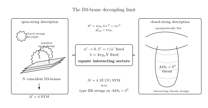
At fixed $g_s$, $N$ and finite boundary energies, the fixed-$U$ limit separates the interacting sectors from free massless fields in the asymptotic bulk. The open-string description also contains a separate free center-of-mass $U(1)$ multiplet. The proposed equivalence concerns interacting $SU(N)$ SYM and the throat theory. This is a diagram of the decoupling argument, with no spatial scale implied.

The controlled supergravity regime

Three expansion parameters answer different questions. Curvature in string units is organized by

$$\frac{\alpha'}{R^2}=\frac1{\sqrt\lambda}.$$

Large $\lambda$ makes the background weakly curved. The first nonzero higher-derivative correction to a particular observable depends on the action and its symmetries; it need not start at the first power of this parameter.

Perturbative string loops are controlled by

$$g_s=\frac{\lambda}{4\pi N}.$$

At fixed $\lambda$, increasing $N$ suppresses successive genera. Taking $N$ and $\lambda$ large together does not automatically make $g_s$ small.

For gravity at the AdS scale, dimensional reduction gives a complementary measure. The physical sphere volume is $\pi^3R^5$, so

$$G_5=\frac{G_{10}}{\pi^3R^5}, \qquad \frac{G_5}{R^3}=\frac{\pi}{2N^2}.$$

The coefficient of the classical five-dimensional action is therefore of order $N^2$. Its loop expansion at fixed AdS-scale energies is organized by $1/N^2$. This gravitational expansion and the string genus expansion are related, but $G_5/R^3$ and $g_s^2$ are distinct quantities.

A useful sufficient corner for weakly coupled, weakly curved type IIB supergravity is

$$1\ll\lambda\ll4\pi N, \qquad N\gg1.$$

At weak $\lambda$, planar SYM may be tractable but its string dual is highly curved. At large $\lambda$ in the corner above, the gauge theory is strongly coupled while two-derivative gravity becomes useful. This is an approximation to the proposed duality, rather than its definition.

Radial position and three energy measurements

The Poincaré metric is invariant under

$$x^a\longrightarrow a\,x^a, \qquad z\longrightarrow a\,z.$$

Boundary energies transform inversely. This implies that a scale associated with radial position is proportional to $1/z$, but the symmetry alone does not determine which physical experiment defines that scale.

For a massless Euclidean bulk wave of boundary momentum magnitude $k$, the radial equation is

$$z^2\psi_k''-3z\psi_k'-k^2z^2\psi_k=0.$$

Its radial dependence is controlled by $kz$. Boundary variations of wavelength $1/k$ appreciably probe depths of order $z\sim1/k$. The corresponding resolution scale is therefore

$$\mu\sim\frac1z=\frac{U}{\sqrt\lambda}.$$

A concrete position-space example is the regular response to a point source for a massless scalar in Euclidean $AdS_5$:

$$K_4(z,\rho)=\frac6{\pi^2}\frac{z^4}{(z^2+\rho^2)^4}, \qquad \rho=|x-x'|, \qquad \int d^4x\,K_4(z,|x|)=1.$$

The kernel becomes a delta function as $z\to0$. At finite depth its normalized shape depends only on $\rho/z$. It makes the relation between depth and spatial resolution explicit; it is not a universal profile for arbitrary bulk objects. The construction follows the massless example in Witten, section 2.4.

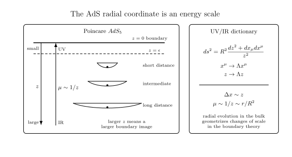
The curves plot $K_4(z,\rho)/K_4(z,0)=[1+(\rho/z)^2]^{-4}$ for $z=z_0$ and $z=2z_0$, with a common horizontal scale $\rho/z_0$. Their half-height radii are $\rho_{1/2}=z\sqrt{2^{1/4}-1}\simeq0.435z$. Only the finite interval shown is plotted. The normalized shape illustrates the wave-resolution relation $\mu\sim1/z$; the vertical axis is neither a probability density nor an energy.

Now perform a different experiment. Stretch a static fundamental string radially from the stack to a probe brane. The string action measures the energy in the coordinate $t$ through

$$E_{\rm string} =\frac1{2\pi\alpha'}\int_0^r dr'\sqrt{-g_{tt}g_{rr}} =\frac r{2\pi\alpha'}=\frac U{2\pi},$$

because the two warp factors cancel. This is the mass of a stretched-string W boson on the Coulomb branch. It differs from the wave-resolution scale by a factor proportional to $\sqrt\lambda$.

Together with the local oscillator considered above, the three measurements give

Measurement	Boundary energy scale at fixed $U$
Bulk wave resolving a region of size $z$	$\mu\sim U/\sqrt\lambda$
Local string-scale excitation	$E\sim U/\lambda^{1/4}$
String stretched from the stack to a probe	$m_W=U/(2\pi)$

There is no contradiction: the probes are different. Peet and Polchinski, section 1.1, explain why the stretched-string mass should not be substituted for the holographic resolution scale. Radial position organizes scale dependence, but an exact Wilsonian interpretation requires specifying the observable and the cutoff procedure.

Boundary sources and the renormalized action

The GKPW prescription turns the correspondence into a proposal for generating observables. Its original formulations are due to Gubser, Klebanov and Polyakov and Witten.

Consider a scalar in $AdS_5$. Near the boundary, the terms without boundary derivatives determine the powers: substituting $\psi\sim z^q$ into the wave equation gives

$$q(q-4)=m^2R^2.$$

In standard quantization, write $\Delta=2+\sqrt{4+m^2R^2}$ and schematically

$$\psi(z,x) =z^{4-\Delta}\bigl[J(x)+\cdots\bigr] +z^\Delta\bigl[A(x)+\cdots\bigr].$$

The source is the coefficient $J$, with mass dimension $4-\Delta$. It is generally not the literal value of $\psi$ at $z=0$: that value may vanish or diverge. Local derivative terms and, at special exponents, logarithms must be included in a complete expansion. Their treatment and the allowed alternative boundary conditions are developed on page 32.

For a massless scalar, the two powers are $z^0$ and $z^4$. A dimensionless source couples to a dimension-four operator, as for the dilaton. The exponent zero identifies the source behavior; it does not give a second allowed dimension-zero dilaton operator.

With the shared Euclidean convention, the proposed equality is

$$Z_{\rm IIB}[J] =Z_{\rm CFT}[J] =\left\langle\exp\!\left(\int d^4x\,J\mathcal O\right)\right\rangle.$$

At a classical saddle with the prescribed asymptotic source and a chosen interior condition,

$$W_E[J]\equiv\log Z_{\rm CFT}[J] \simeq-S_{E,\rm ren}[\psi_{\rm cl}[J]].$$

The subscript “ren” is essential. To see why, start with a scalar action

$$S_E=\frac{\mathcal N}{2}\int d^5x\sqrt g\, \bigl[(\partial\psi)^2+m^2\psi^2\bigr].$$

After integrating by parts and imposing the equation of motion, the regulated action has the boundary term

$$S_{E,\rm reg}^{\rm os} =\frac{\mathcal N}{2}\int_{z=\epsilon}d^4x\sqrt\gamma\, \psi\,n^M\partial_M\psi, \qquad n^M\partial_M=-\frac zR\partial_z.$$

The normal points out of the region $z\ge\epsilon$, toward decreasing $z$. Because $\sqrt\gamma=R^4/\epsilon^4$, the boundary term can diverge even when the field has a well-defined source coefficient. Local counterterms built from the induced fields cancel these divergences:

$$S_{E,\rm ren}[J] =\lim_{\epsilon\to0} \left(S_{E,\rm reg}^{\rm os}+S_{E,\rm ct}\right).$$

The limiting procedure holds the renormalized source fixed. De Haro, Skenderis and Solodukhin, section 5.1, give the systematic scalar construction. Exercise 5 carries it out for an elementary solution where the cancellation is exact at finite cutoff.

Functional derivatives now give

$$\begin{aligned} \langle\mathcal O(x)\rangle_J &=\frac{\delta W_E}{\delta J(x)} =-\frac{\delta S_{E,\rm ren}}{\delta J(x)},\\ \langle\mathcal O(x)\mathcal O(y)\rangle_{\rm conn} &=\left.\frac{\delta^2W_E}{\delta J(x)\delta J(y)}\right|_{J=0}. \end{aligned}$$

The coefficient $A$ encodes the response; its proportionality to the one-point function is fixed by the bulk kinetic normalization and the renormalized variation. Adding a finite local functional of $J$ changes contact terms. It leaves separated-point nonlocal correlations unchanged. These statements fix the sign and normalization procedure; they do not leave an arbitrary sign to choose after computing a correlator.

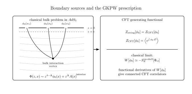
For a standard-quantized scalar near the Euclidean AdS vacuum, fix the asymptotic source coefficient, solve with regular interior behavior, and renormalize the regulated action before differentiating. The cutoff value $\psi(\epsilon,x)$ must be related to $J(x)$. Finite local counterterms specify contact terms. The diagram describes a calculation, rather than a guarantee of a unique saddle for arbitrary sources.

The source and the state are distinct data. Euclidean vacuum correlators select the regular interior solution. A real-time response needs an appropriate Lorentzian prescription, such as the ingoing condition used in the absorption calculation. For large sources, backreaction or competing saddles may change the problem. In particular, finite irrelevant sources can alter AdS asymptotics; operator insertions can instead be defined perturbatively by derivatives about zero source.

Symmetry and the first operator families

The bosonic symmetry algebras agree:

$$\mathfrak{so}(2,4)\oplus\mathfrak{so}(6).$$

The first is the four-dimensional conformal algebra. The second rotates the six scalar fields. On spinors the relevant cover is $\operatorname{Spin}(6)\cong SU(4)$; $SO(6)$ and $SU(4)$ are not identical global groups. Including the 16 ordinary and 16 conformal supercharges gives $\mathfrak{psu}(2,2|4)$. Symmetry matching constrains the dictionary but does not establish the duality by itself.

Some basic source/operator pairs are:

Boundary source	CFT operator or response
Boundary metric	Stress tensor
Dimensionless dilaton fluctuation	Full supersymmetric gauge-coupling operator
RR axion	Topological-density operator
R-symmetry gauge field	$SU(4)_R$ current
A specified Kaluza–Klein scalar mode	Scalar operator with the matching mass and R-symmetry representation

For the dilaton and axion, expressions such as $\operatorname{tr}F^2$ and $\operatorname{tr}F\wedge F$ indicate the relevant gauge-field terms. Source variation, including the action’s prefactors and its supersymmetric completion, defines the actual normalized operators. The dilaton absorption calculation illustrates why a free quadratic expression does not by itself define the complete interacting operator.

The last row requires care. Expanding a minimally coupled ten-dimensional dilaton in degree-$\ell$ scalar harmonics on $S^5$ gives

$$m_\ell^2R^2=\ell(\ell+4), \qquad \Delta_\ell=\ell+4, \qquad \ell=0,1,2,\ldots.$$

A different protected family consists of the symmetric traceless chiral primaries

$$\mathcal O_k^{I_1\cdots I_k} \sim\operatorname{tr}\bigl(X^{(I_1}\cdots X^{I_k)}\bigr)-\text{traces}, \qquad \Delta=k, \qquad k\ge2.$$

These correspond to particular mixed metric/five-form modes with

$$m_k^2R^2=k(k-4).$$

This mixed-family mass is a result of the Kaluza–Klein analysis, not the eigenvalue of a free dilaton harmonic. The distinction and the protected dimensions are discussed in Witten, section 2.5. For $SU(N)$, the $k=1$ trace vanishes. At finite $N$, trace relations and mixing with multiparticle operators also prevent treating all single-trace expressions as an independent infinite tower.

The source prescription thus requires more than matching a field’s name: one must specify its harmonic, its mixing with other fields, its boundary condition and its normalization. The next page develops the scalar boundary problem that makes these identifications calculable.

Common pitfalls

Taking the boundary limit before isolating the throat. At finite $\alpha'$, the original geometry becomes flat at large $r$. The complete AdS boundary belongs to the fixed-$U$ limiting geometry, whose neck has moved to $U=\infty$.

Calling every radial energy scale $U$. The stretched-string mass, local oscillator energy and bulk-wave resolution scale have different dependence on $\lambda$. Specify the physical probe before assigning an energy to a radial position.

Differentiating a divergent action. The cutoff action and the renormalized source functional are different objects. The outward normal, local counterterms and the quantity held fixed all enter the response calculation.

Identifying all sphere scalars with chiral primaries. The minimal dilaton tower and the mixed metric/five-form tower have different masses and dimensions. The harmonic representation alone does not identify the full bulk mode.

Exercises

1. How uniform is the fixed-U approximation?

On $0<U\le U_{\max}$, find a sufficient condition on $\alpha'$ for the relative errors of all three rescaled metric coefficients to be at most $\eta>0$. Compare the limits at fixed $U$, fixed nonzero $r$, and $U=c/\sqrt{\alpha'}$ with fixed $c>0$.

Solution

The radial and sphere coefficients differ from their throat values by the factor $\sqrt{1+\delta}$; the worldvolume coefficient differs by its inverse. For $\delta\ge0$,

$$\sqrt{1+\delta}-1 =\frac\delta{\sqrt{1+\delta}+1}\le\frac\delta2,$$

and

$$1-\frac1{\sqrt{1+\delta}} =\frac\delta{\sqrt{1+\delta}\,[\sqrt{1+\delta}+1]} \le\frac\delta2.$$

It is therefore sufficient that

$$\frac{\alpha'^2U_{\max}^4}{\lambda}\le2\eta, \qquad \alpha'\le\frac{\sqrt{2\eta\lambda}}{U_{\max}^2}.$$

The last expression has units of length squared. The approximation is uniform on this bounded range of $U$, although the coordinate coefficient of $dU^2$ itself diverges as $U\to0$.

At fixed $U$, $\delta\to0$. At fixed nonzero $r$, instead, $H=1+\lambda\alpha'^2/r^4\to1$. For $U=c/\sqrt{\alpha'}$, the correction remains $\delta=c^4/\lambda$: it does not vanish. This scaling follows the transition region when $c$ is of order $\lambda^{1/4}$. The limit is consequently not uniform over all $0<U<\infty$ at once.

2. Three probes at a radial position

Compute the static string energy between two radially aligned probe positions $U_1<U_2$. Compare the mass of a string from the stack to $U$ and the energy of a local oscillator with the wave-resolution scale $\mu\sim U/\sqrt\lambda$. Why would integrating only proper radial length give the wrong boundary energy?

Solution

In static gauge $(\tau,\sigma)=(t,r)$, the induced determinant is $g_{tt}g_{rr}=-1$. Thus

$$E_{12}=\frac1{2\pi\alpha'}\int_{r_1}^{r_2}dr =\frac{U_2-U_1}{2\pi}.$$

Taking $U_1=0$ gives $m_W=U/(2\pi)$. The proper string length contains $\sqrt{g_{rr}}\,dr$, but a proper energy must also be multiplied by $\sqrt{-g_{tt}}$ to obtain its energy conjugate to $t$. Those factors cancel. Using proper length alone omits the redshift.

For a local oscillator with $E_{\rm local}=c_s/\sqrt{\alpha'}$, the throat metric gives $E_{\rm osc}=c_sU/\lambda^{1/4}$. If the representative wave scale is chosen as $1/z$, the ratios are

$$\frac{m_W}{1/z}=\frac{\sqrt\lambda}{2\pi}, \qquad \frac{E_{\rm osc}}{1/z}=c_s\lambda^{1/4}.$$

All three energies transform inversely under a boundary dilation, but scale covariance leaves these coupling-dependent ratios undetermined. The W boson is an extended string probe; it need not have the energy of a supergravity wave that resolves the same radial depth.

3. Gravity loops, string loops and curvature

Derive $G_5/R^3$ from the ten-dimensional Newton constant. For the double scaling $\lambda=N^\beta$, determine when $\lambda\to\infty$ and $g_s\to0$ simultaneously. Finally, compute the scalar curvature and the squared Riemann tensor of $AdS_5\times S^5$ to explain why a vanishing total scalar curvature does not imply a flat background.

Solution

The shared gravitational coupling gives

$$G_{10}=8\pi^6g_s^2\alpha'^4.$$

Since the sphere volume is $\pi^3R^5$ and $R^8=16\pi^2g_s^2N^2\alpha'^4$,

$$\frac{G_5}{R^3} =\frac{G_{10}}{\pi^3R^8} =\frac{\pi}{2N^2}.$$

For $\lambda=N^\beta$,

$$\frac{\alpha'}{R^2}=N^{-\beta/2}, \qquad g_s=\frac1{4\pi}N^{\beta-1}.$$

Both desired limits hold for $0<\beta<1$. At $\beta=1$, the string coupling approaches a constant; at $\beta>1$ it grows. By contrast, $G_5/R^3$ tends to zero in all these cases. This makes explicit why the gravity-loop parameter at the AdS scale and the perturbative string coupling must be distinguished.

For an $n$-dimensional constant-curvature space of sectional curvature $K$,

$$\mathcal R=n(n-1)K, \qquad \mathcal R_{abcd}\mathcal R^{abcd}=2n(n-1)K^2.$$

The two factors have $n=5$ and $K=\mp1/R^2$. Their scalar curvatures cancel, while their squared curvatures add:

$$\mathcal R_{10}=0, \qquad \mathcal R_{MNPQ}\mathcal R^{MNPQ}=\frac{80}{R^4}.$$

The local curvature scale remains $1/R^2$. A vanishing scalar contraction alone cannot eliminate higher-derivative effects.

4. Two different scalar towers

Separate the minimally coupled ten-dimensional scalar equation using a degree-$\ell$ harmonic with $-\nabla^2_{S^5}Y_\ell=\ell(\ell+4)Y_\ell/R^2$. Find the standard operator dimension. Compare its $\ell=2$ mode with the mixed metric/five-form mode whose supplied mass is $m_k^2R^2=k(k-4)$ at $k=2$.

Solution

For $\psi(x,z,\Omega)=\psi_\ell(x,z)Y_\ell(\Omega)$, the product Laplacian yields

$$\left(\nabla^2_{AdS_5}-\frac{\ell(\ell+4)}{R^2}\right)\psi_\ell=0.$$

The standard dimension is

$$\Delta_\ell=2+\sqrt{4+\ell(\ell+4)} =2+(\ell+2)=\ell+4.$$

Thus the $\ell=2$ dilaton harmonic has $m^2R^2=12$ and $\Delta=6$. The supplied mixed-family result at $k=2$ instead gives $m^2R^2=-4$ and $\Delta=2$, the dimension of the symmetric traceless bilinear chiral primary. This mode sits at the scalar stability bound; its coincident radial exponents require the special boundary analysis developed on the next page.

The difference arises because the latter fluctuation involves coupled metric and five-form fields. A scalar harmonic labels its R-symmetry representation, but does not remove those couplings. The displayed mixed mass is input from that coupled analysis, not a consequence of the minimal scalar equation just solved. The restriction $k\ge2$ also agrees with $\operatorname{tr}X^I=0$ in $SU(N)$; the free center-of-mass mode belongs to the separate $U(1)$ sector.

5. An elementary renormalized response

Consider a real, dimensionless toy scalar $\psi$ in Euclidean $AdS_5$, with dimensionless $C$ and action

$$S_E=\frac{C}{2R^3}\int d^5x\sqrt g\, \bigl[(\partial\psi)^2+m^2\psi^2\bigr], \qquad C>0, \qquad m^2R^2=-\frac{15}{4}.$$

Choose standard quantization, $\Delta=5/2$. For Euclidean momentum magnitude $k>0$, verify that $\psi(z,k)=z^{3/2}e^{-kz}J(k)$ is regular and compute the renormalized action. Use the counterterm

$$S_{E,\rm ct}=\frac{C}{2R^3}\int_{z=\epsilon}d^4x\sqrt\gamma\, \frac{3}{2R}\psi^2.$$

Distinguish the asymptotic source $J$ from $J_\epsilon=\epsilon^{-3/2}\psi(\epsilon)$. Find the momentum-space and separated-point two-point functions. This scalar is an illustrative boundary problem, with no identification as a particular IIB mode assumed.

Solution

The radial equation is

$$z^2\psi_k''-3z\psi_k'-k^2z^2\psi_k+\frac{15}{4}\psi_k=0.$$

Direct differentiation verifies the stated solution. It decays at large $z$ for $k>0$, and its near-boundary expansion is

$$\psi=z^{3/2}J-kz^{5/2}J+\cdots, \qquad A=-kJ.$$

Write $\int_k=\int d^4k/(2\pi)^4$. With outward normal $n=-z\partial_z/R$, the regulated boundary action is

$$S_{E,\rm reg}^{\rm os} =\frac C2\int_k e^{-2k\epsilon}J(k)J(-k) \left(k-\frac{3}{2\epsilon}\right).$$

The counterterm gives

$$S_{E,\rm ct} =\frac C2\int_k e^{-2k\epsilon}J(k)J(-k) \frac{3}{2\epsilon}.$$

It cancels the divergence before the cutoff is removed. At fixed asymptotic $J$,

$$S_{E,\rm ren} =\frac C2\int_k kJ(k)J(-k).$$

At finite cutoff, $J_\epsilon=e^{-k\epsilon}J$. The sum of the two regulated terms is exactly $C\int_k kJ_\epsilon(k)J_\epsilon(-k)/2$. Taking source derivatives of this expression uses $J_\epsilon$ as the independent source; using $J$ as the independent source in the earlier expression retains the exponential factors. Both procedures give the same limit when their source relation is included.

Since $W_E=-S_{E,\rm ren}$, the two-point function, with its momentum-conserving delta function stripped off, is

$$G_E(k)=-C|k|.$$

Its negative momentum coefficient does not imply a negative separated-point coefficient. As a distribution defined by analytic continuation, the Fourier identity in four dimensions is

$$\int\frac{d^4k}{(2\pi)^4}e^{ik\cdot x}(k^2)^\nu =\frac{4^\nu\Gamma(2+\nu)}{\pi^2\Gamma(-\nu)} \frac1{|x|^{4+2\nu}}, \qquad x\ne0.$$

At $\nu=1/2$, the coefficient is $-3/(4\pi^2)$. Therefore

$$\langle\mathcal O(x)\mathcal O(0)\rangle =\frac{3C}{4\pi^2|x|^5}, \qquad x\ne0.$$

The source has mass dimension $3/2$, the operator has dimension $5/2$, and $C$ is dimensionless in the specified action. Local finite terms would alter the coincident-point distribution, not this coefficient. The Fourier integral is not an absolutely convergent ordinary integral; interpreting it that way would invalidate the calculation.

6. Normalizations, contact terms and profile widths

Rescale a source and operator by $J'=aJ$ and $\mathcal O'=\mathcal O/a$, with real nonzero $a$. Track the two-point coefficient. Then add $\frac12\int d^4x[c_0J^2+c_2(\partial J)^2]$ to the renormalized action and find its effect. Finally, verify the normalization of $K_4$ and calculate the half-height width plotted above.

Solution

The source coupling is unchanged, $J'\mathcal O'=J\mathcal O$. The new functional is $W'[J']=W[J'/a]$, so two derivatives give

$$G'_E=\frac1{a^2}G_E.$$

This is a change in operator normalization. The local addition to $S_{E,\rm ren}$ instead changes the two-point function by

$$\delta G_E(k)=-c_0-c_2k^2.$$

Its position-space support is at coincident points, through a delta function and its derivatives. It changes the contact-term scheme but does not rescale the separated-point tail. Neither operation changes a length scale in a specified bulk solution.

For the kernel, the four-dimensional angular measure is $2\pi^2\rho^3d\rho$. Setting $v=\rho/z$ gives

$$\int d^4x\,K_4 =12\int_0^\infty\frac{v^3\,dv}{(1+v^2)^4} =6\int_0^\infty\frac{t\,dt}{(1+t)^4}=1,$$

where the last integral is $B(2,2)=1/6$. Its peak-normalized profile is $(1+\rho^2/z^2)^{-4}$. Setting it equal to $1/2$ yields

$$\rho_{1/2}=z\sqrt{2^{1/4}-1}\simeq0.434979442\,z.$$

Doubling $z$ doubles this width. This is a calculable change in the spatial profile of this particular Euclidean source response. Peak normalization was used only to compare the two plotted shapes; the full kernel separately obeys the unit-integral normalization just verified.

References

• Sebastian de Haro, Kostas Skenderis and Sergey N. Solodukhin, “Holographic Reconstruction of Spacetime and Renormalization in the AdS/CFT Correspondence,” Communications in Mathematical Physics 217 (2001), 595–622. doi:10.1007/s002200100381; arXiv:hep-th/0002230.
• Steven S. Gubser, Igor R. Klebanov and Alexander M. Polyakov, “Gauge Theory Correlators from Non-Critical String Theory,” Physics Letters B 428 (1998), 105–114. doi:10.1016/S0370-2693(98)00377-3; arXiv:hep-th/9802109.
• Juan M. Maldacena, “The Large N Limit of Superconformal Field Theories and Supergravity,” Advances in Theoretical and Mathematical Physics 2 (1998), 231–252. arXiv:hep-th/9711200.
• Amanda W. Peet and Joseph Polchinski, “UV/IR Relations in AdS Dynamics,” Physical Review D 59 (1999), 065011. doi:10.1103/PhysRevD.59.065011; arXiv:hep-th/9809022.
• Edward Witten, “Anti De Sitter Space and Holography,” Advances in Theoretical and Mathematical Physics 2 (1998), 253–291. arXiv:hep-th/9802150.