Type IIB S-Duality, (p,q) Strings, and the D3-Brane

Type IIB duality relates a fundamental string to a D-string, and an electrically charged particle on a D3-brane to a magnetic monopole. These statements involve more than inverting a coupling: the integer charges, background fields, metric used to measure energy, and allowed line operators must transform together. The central result is the BPS string tension

$$T^{S}_{p,q}=T_{\mathrm{F1}}|p-q\tau|, \qquad \tau=C_0+i e^{-\Phi}.$$

We derive its charge and frame dependence, the associated covariance of the supergravity fields, and the low-energy electromagnetic calculation on a D3-brane. The BPS spectrum and the full interacting string duality supply additional quantum information beyond these calculations. We use the overview’s frames and gravitational couplings, RR potential basis, and D-brane and gauge normalizations. Page 24 supplies the zero-axion charge algebra and compact electric-flux construction.

The axio-dilaton and the integral string lattice

Write $\tau=x+iy$, where $x=C_0$ and $y=e^{-\Phi}>0$. In a constant vacuum, $y=1/g_s$. A real matrix of determinant one acts on the upper half-plane by

$$\Lambda=\begin{pmatrix}a&b\\c&d\end{pmatrix}, \qquad \tau'=\frac{a\tau+b}{c\tau+d}.$$

Direct differentiation and subtraction of the complex conjugate give

$$d\tau'=\frac{d\tau}{(c\tau+d)^2}, \qquad y'=\frac{y}{|c\tau+d|^2}.$$

Thus $d\tau\,d\bar\tau/y^2$ is an invariant metric. The continuous classical covariance becomes an integral duality group when the quantized charge lattice is included.

Let $D_2=C_2^{\mathrm{WZ}}=-C_2$ denote the shared brane-coupling two-form, and define the useful columns $\mathcal B=(B_2,D_2)^T$ and $Q=(p,q)^T$. The string source is $T_{\mathrm{F1}}\int Q^T\mathcal B$. Invariance of this pairing requires

$$Q'=\Lambda Q, \qquad \mathcal B'=\Lambda^{-T}\mathcal B, \qquad \begin{pmatrix}B_2'\\D_2'\end{pmatrix} =\begin{pmatrix}dB_2-cD_2\\-bB_2+aD_2\end{pmatrix}.$$

The primitive electric sources are $(1,0)$ for F1 and $(0,1)$ for D1. Both are electrically charged under ten-dimensional two-forms. Their later interpretation as electric and magnetic particles refers to the four-dimensional D3 gauge field.

Preserving all integer charges and their antisymmetric pairing $pq'-qp'$ restricts $\Lambda$ to $SL(2,\mathbb Z)$. Two generators are

$$S=\begin{pmatrix}0&-1\\1&0\end{pmatrix}, \qquad T=\begin{pmatrix}1&1\\0&1\end{pmatrix}.$$

Here $S$ sends $\tau\to-1/\tau$ and $(p,q)\to(-q,p)$, while $T$ sends $\tau\to\tau+1$ and $(p,q)\to(p+q,q)$. At zero axion, $S$ inverts $g_s$. A positive D1 becomes a negative F1 under this choice of $S$; $S^{-1}$ gives positive F1 instead. Moreover $S^2=-I$ fixes $\tau$ but reverses charges and two-forms. The fractional action on moduli factors through $PSL(2,\mathbb Z)$, whereas oriented charged states retain the central element.

The BPS tension and the axion shift

The identity

$$p'-q'\tau'=\frac{p-q\tau}{c\tau+d}$$

shows how to form an invariant central-charge length:

$$Z_Q=\frac{p-q\tau}{\sqrt y}, \qquad Z_{Q'}'=\frac{|c\tau+d|}{c\tau+d}Z_Q.$$

Only its phase changes. The tension in the invariant, unshifted Einstein metric $\widehat g$ is consequently

$$\widehat T_{p,q}=T_{\mathrm{F1}}|Z_Q|, \qquad T^S_{p,q}=T_{\mathrm{F1}} \sqrt{(p-qC_0)^2+q^2e^{-2\Phi}}.$$

The conversion uses $G_S=e^{\Phi/2}\widehat g$: a two-dimensional induced area gains $e^{\Phi/2}$, so $\widehat T=e^{\Phi/2}T^S$. The BPS algebra fixes the norm once the charges are calibrated; existence of the primitive type IIB strings is additional spectrum information. Schwarz derives the charge multiplet and its tension. Witten’s bound-state analysis distinguishes the one-D1 flux argument from the many-D1 quantum problem.

The plotted charges have $p,q\in\{-1,0,1\}$ before transformation. At $\tau=\tfrac12+i$, $S\tau=-\tfrac25+\tfrac45i$; the transformed labels are $(-q,p)$. Both planes use equal scales, so unchanged lengths represent unchanged $\widehat T/T_{\mathrm{F1}}$. The phase rotation is $-\arg\tau$. Opposite points are oppositely oriented strings, even though $-I$ leaves the modulus fixed.

What the compact D1 actually derives

For one D1 at constant axion and coupling, put $f=2\pi\alpha'$ and $e=fF_{01}$. The DBI and WZ terms give the Lagrangian density

$$\frac{\mathcal L}{T_{\mathrm{F1}}} =-\frac{\sqrt{1-e^2}}{g_s}+C_0e.$$

On a circle of physical circumference $L_c$, the holonomy $a=\int A_1dx^1$ has period $2\pi$. For a homogeneous field, $e=f\dot a/L_c$, and $T_{\mathrm{F1}}f=1$ makes its canonical momentum

$$P_a=\frac{\partial(L_c\mathcal L)}{\partial\dot a} =C_0+\frac{e}{g_s\sqrt{1-e^2}}=p\in\mathbb Z.$$

The integer follows from periodic wavefunctions $e^{ipa}$, not from a classical quantization of $e$. Solving for $e$ and making the Legendre transform yields

$$e=\frac{g_s(p-C_0)}{\sqrt{1+g_s^2(p-C_0)^2}}, \qquad \frac{\mathcal H}{T_{\mathrm{F1}}} =\sqrt{(p-C_0)^2+g_s^{-2}}.$$

The kinetic DBI displacement is $p-C_0$, whereas the full conserved source for $B_2$ is $pT_{\mathrm{F1}}$: the WZ term also varies with $B_2+fF$. Under $T$, $p\to p+1$ and $C_0\to C_0+1$, leaving the kinetic combination unchanged. Varying $C_0$ with $p$ held fixed is a different operation and generally changes the energy. For general $q$, the corresponding combination is $p-qC_0$; the single Abelian rotor does not establish the existence of every multi-D1 bound state.

A primitive vector has $\gcd(p,q)=1$ and lies in the integral orbit of F1. If $Q=kQ_0$, its BPS tension is $|k|$ times that of $Q_0$, allowing threshold splitting. The triangle inequality also gives $\widehat T_{Q_1+Q_2}\leq\widehat T_{Q_1}+\widehat T_{Q_2}$. Neither statement alone proves a normalizable bound state. At a string junction, oriented charge conservation is $\sum_iQ_i=0$; a supersymmetric static junction additionally requires spatial force balance and compatible preserved supercharges.

Covariant fields and the nonlinear five-form

The distinction between fields and charges can be expressed by a positive matrix derived from the three-form norm:

$$\mathcal M(\tau)=\frac1y \begin{pmatrix}|\tau|^2&x\\x&1\end{pmatrix}, \qquad \mathcal M^{-1}=\frac1y \begin{pmatrix}1&-x\\-x&|\tau|^2\end{pmatrix}.$$

Let $H_3=dB_2$, $K_3=dD_2$, and $\mathcal G_3=K_3+\tau H_3$. Expanding its square gives

$$\frac{|\mathcal G_3|^2}{y} =y|H_3|^2+\frac{|K_3+xH_3|^2}{y}, \qquad Q^T\mathcal M^{-1}Q=\frac{|p-q\tau|^2}{y}.$$

Thus the field quadratic form uses $\mathcal M$ and the charge quadratic form uses its inverse. Substitution of the transformed two-forms gives $\mathcal G_3'=\mathcal G_3/(c\tau+d)$, or equivalently $\mathcal M'=\Lambda\mathcal M\Lambda^T$. In the unshifted Einstein formulation, the scalar and three-form terms inside the common $1/(2\kappa_{10,0}^2)$ action are

$$-\frac{\partial\tau\cdot\partial\bar\tau}{2y^2} -\frac{|\mathcal G_3|^2}{2y}.$$

Both are invariant with $\widehat g$ held fixed. The norm includes the usual form factorial. In the bulk basis, $K_3+C_0H_3=-\widetilde F_3$, which explains the otherwise easy-to-miss relative sign. These are two terms of the IIB pseudo-action; its five-form constraint and Chern–Simons term still have to be included as in page 11.

The symmetric bulk four-form $C_4$ may be held invariant under a constant $\Lambda$. Its field strength is

$$\widetilde F_5=dC_4+\frac12(D_2\wedge H_3-B_2\wedge K_3).$$

The bilinear in parentheses is invariant because $ad-bc=1$. This works for nonconstant two-forms; no assumption $H_3=K_3=0$ was used. But the WZ four-form $D_4=C_4^{\mathrm{WZ}}=C_4-\tfrac12B_2\wedge D_2$ is not itself a singlet. Its required transformation is

$$D_4'=D_4+\frac{bd}{2}B_2\wedge B_2 +\frac{ac}{2}D_2\wedge D_2-bcB_2\wedge D_2.$$

Indeed $\widetilde F_5=dD_4+H_3\wedge D_2$ remains unchanged. Also $d\widetilde F_5=-H_3\wedge K_3$ remains unchanged, and the imposed equation $\widetilde F_5=*\widetilde F_5$ is compatible with the invariant metric. The nonlinear RR basis matters whenever two-form fields are present; the WZ expansion and bulk strengths in Myers, equations (3)–(5) translate to this shared basis.

Frames and a D1-to-F1 background

In a constant vacuum put $s=|c\tau+d|$. The dilaton law gives $g_s'=s^2g_s$, and invariance of $\widehat g$ gives

$$G_S'=sG_S,\qquad L_S'=\sqrt{s}\,L_S,\qquad T_S'=\frac{T_S}{s},\qquad M_S'=\frac{M_S}{\sqrt{s}}.$$

The last relation follows either from a particle’s proper-time action or from $M_S=L_ST_S$ for a straight stretched string. A mass is not a tension: they have different frame weights. The separately asymptotically normalized Einstein metrics satisfy $g'=sg$, whereas $\widehat g'=\widehat g$. In each constant vacuum,

$$L_{\widehat g}=g_s^{-1/4}L_S, \qquad M_{\widehat g}=g_s^{1/4}M_S, \qquad T_{\widehat g}=g_s^{1/2}T_S.$$

For a D3, its four-dimensional induced volume instead gains $e^{\Phi}$; hence its unshifted Einstein tension is $\widehat T_3=\mu_3$, independent of the coupling. Its tension in the shared asymptotically normalized frame is $T_3=\mu_3/g_s$. These statements use the two distinct metrics already defined in the overview.

As a local supergravity illustration, consider the D1 exterior solution with vanishing axion:

$$\begin{aligned} ds_S^2&=H^{-1/2}ds_\parallel^2+H^{1/2}ds_\perp^2,\\ e^\Phi&=g_sH^{1/2},\qquad H(r)=1+(R/r)^6. \end{aligned}$$

Since $|\tau|=e^{-\Phi}$, applying $S$ gives

$$ds_S'^2=g_s^{-1}\bigl(H^{-1}ds_\parallel^2+ds_\perp^2\bigr), \qquad e^{\Phi'}=g_s^{-1}H^{-1/2}.$$

This has the F1 metric and dilaton profile, with opposite F1 orientation for the displayed $S$. To restore unit asymptotic metric components, set $x'^\mu=x^\mu/\sqrt{g_s}$; the transformed harmonic radius is $R'=R/\sqrt{g_s}$. The absolute relation between $R$, charge and coupling belongs to the supergravity solutions on page 26. The transformation does not ensure small curvature and small local coupling at every radius.

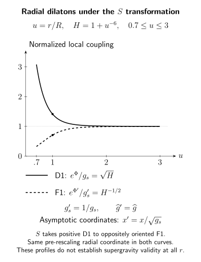
The exact plotted functions are $\sqrt{1+u^{-6}}$ and its inverse for $u=r/R\in[0.7,3]$. They use the same radial coordinate before asymptotic rescaling, and are normalized by $g_s$ and $g_s'=1/g_s$ respectively. The metric and dilaton do not distinguish F1 orientation; the charge transformation fixes it. This local background example does not assert supergravity validity over the entire plotted interval.

The D3 gauge action and electromagnetic duality

Deriving the two gauge couplings

Expand the D3 DBI determinant about a constant vacuum and zero background two-forms. The identity $\operatorname{tr}(\eta^{-1}F)=0$ gives

$$\sqrt{-\det(\eta+fF)}=1+\frac{f^2}{4}F_{ab}F^{ab}+O(F^4).$$

For a stack, the quadratic action and WZ term are therefore

$$S_{\mathrm{quad}}=-\frac{\mu_3f^2}{4g_s}\int d^4x\,\operatorname{tr}F_{ab}F^{ab} +\frac{\mu_3f^2 C_0}{2}\int\operatorname{tr}(F\wedge F).$$

Using $\mu_3f^2=1/(2\pi)$ and the shared fundamental trace gives

$$g_{\mathrm{YM}}^2=4\pi g_s,\qquad \theta=2\pi C_0,\qquad \tau_{\mathrm{YM}}=\frac{\theta}{2\pi}+\frac{4\pi i}{g_{\mathrm{YM}}^2}=\tau.$$

For a single brane with a unit-charge Abelian connection, the ordinary numerical field strength replaces the matrix trace. Matching $-F_{ab}F^{ab}/(4g_A^2)$ instead gives $g_A^2=2\pi g_s$. Its complex coupling is $C_0+2\pi i/g_A^2$. The factor of two is a normalization of generators and charges, not two predictions for the same action.

The local dual equations and their charge orientation

For the Abelian field the Lorentzian quadratic action becomes

$$S_L=-\frac1{4\pi}\int\bigl[yF\wedge *F-xF\wedge F\bigr].$$

Here the star is the induced four-dimensional Lorentzian star. Define the derived constitutive two-form $G=xF-y*F$. Since $\delta S_L=(2\pi)^{-1}\int\delta F\wedge G$, the source-free equations are $dF=dG=0$. The transformation

$$\begin{pmatrix}G'\\F'\end{pmatrix} =S\begin{pmatrix}G\\F\end{pmatrix} =\begin{pmatrix}-F\\G\end{pmatrix}$$

preserves these equations and gives the same constitutive law at $\tau'=-1/\tau$. To verify it, use $*^2=-1$ on two-forms and invert $F'=xF-y*F$. The coefficient of $*F'$ is $-y/|\tau|^2$, and that of $F'$ is $-x/|\tau|^2$.

The integral normalization can be seen directly in a first-order path integral. After Euclidean continuation, $*^2=1$ and

$$I_1[F,F_D]=\frac1{4\pi}\int \bigl[yF\wedge *F-ixF\wedge F+2iF\wedge F_D\bigr].$$

Initially $F$ is an independent real two-form. The dual field $F_D$ is a curvature with periods $2\pi\mathbb Z$. Integration over its continuous potential imposes $dF=0$; summing its integral fluxes imposes the integral periods of $F/(2\pi)$ through a Fourier sum. Thus the mixed coefficient is $i/(2\pi)$, not an adjustable convention after the charge unit has been fixed.

Varying $F$ and solving the resulting Gaussian equation gives

$$y*F-ixF+iF_D=0, \qquad F=\frac{xF_D-iy*F_D}{x^2+y^2}.$$

Substitution yields

$$I_D=\frac1{4\pi}\int \left[\frac{y}{|\tau|^2}F_D\wedge *F_D +i\frac{x}{|\tau|^2}F_D\wedge F_D\right].$$

This is precisely $\tau_D=-1/\tau$. The sign of the mixed term is the Wick rotation of $-(2\pi)^{-1}\int F\wedge F_D$ in the Lorentzian first-order action, where its equation sets $F_D=G$. Reversing that sign reverses the orientation of the dual charge unit without changing the Gaussian coupling inversion.

This is the first-order method of Witten, section 2.2, with the Euclidean theta sign translated to the present Lorentzian WZ coupling. The field-independent Gaussian determinant and sums over topology matter for a complete curved-space partition function; the local calculation alone does not establish modular invariance on every four-manifold. It also does not prove non-Abelian S-duality.

Stretched strings, monopoles, and signed charges

Take two D3-branes separated in one transverse direction by a string-frame proper distance $L$. In the low-energy matrix scalar $\Phi_Y=Y/f$, remove the common position and write $\langle\Phi_Y\rangle=vT^3$, where $v=L/f$ and $T^3=\operatorname{diag}(1,-1)/2$. The eigenvalue difference is $v$, not $2v$.

The kinetic term $-g_{\mathrm{YM}}^{-2}\operatorname{tr}(D\Phi_Y)^2$ contains $[A,vT^3]$. Since $[T^3,T^\pm]=\pm T^\pm$, comparison with the gauge kinetic term gives $M_W=v$. A stretched F1 gives exactly $LT_{\mathrm{F1}}=v$.

For a static dyon, put $E_i=F_{0i}$ and $B_i=\tfrac12\epsilon_{ijk}F_{jk}$. With $D_0\Phi_Y=0$ and Gauss’ law, the energy may be completed as

$$\begin{aligned} E={1\over g_{\mathrm{YM}}^2}\int d^3x\, \operatorname{tr}\bigl[(E_i-\sin\chi D_i\Phi_Y)^2 +(B_i-\cos\chi D_i\Phi_Y)^2\bigr]\\ +{2\over g_{\mathrm{YM}}^2}\oint dS_i\, \operatorname{tr}\bigl[\Phi_Y(\sin\chi E_i+\cos\chi B_i)\bigr]. \end{aligned}$$

In obtaining the surface term, use $D_iB_i=0$ and the static Gauss constraint; a smooth dyon has no prescribed delta-function source at its core. The Abelian fields at large radius determine the charges.

Their signs can be calibrated with the stretched-string picture. Orient a positive $(p,q)$ string from the lower-position brane to the upper-position brane, with worldsheet orientation $dt\wedge d\sigma$. The upper endpoint then carries source $-(p,q)$, because its boundary orientation is $-dt$. For the shared $F_{0i}$ and endpoint coupling $q_{\rm end}\int A$, varying $A_0$ gives outward electric displacement flux $-q_{\rm end}$.

The magnetic sign follows from the D3 WZ term, not from the mass formula. Its coefficient is

$$\mu_3 f\int D_2\wedge F =\frac{\mu_1}{2\pi}\int D_2\wedge F.$$

Under $D_2\to D_2+d\lambda_1$, its variation is $\mu_1(2\pi)^{-1}\int\lambda_1\wedge dF$. Cancellation against a D1 endpoint of charge $q_{D,\rm end}$ requires $dF=-2\pi q_{D,\rm end}\delta_3$. Thus on the upper brane the outward fluxes are

$$\frac1{2\pi}\oint F=q, \qquad \frac1{2\pi}\oint G=p.$$

For example, $G$ has spatial components $(x\mathbf B+y\mathbf E)\cdot d\mathbf S$. The source charge and outward flux have opposite signs in these definitions; exchanging the endpoints reverses both $p$ and $q$.

In the $SU(2)$ Cartan component, the upper brane has $F^3/2$; equivalently, writing simply $F=F^3T^3$ gives

$$\oint B^3_i dS_i=4\pi q, \qquad \frac1{g_{\mathrm{YM}}^2}\oint E^3_i dS_i=p-q\frac{\theta}{2\pi}.$$

The second equation follows from the canonical displacement on that eigenvalue: $\Pi_i^{\rm upper}=E_i^3/g_{\mathrm{YM}}^2+\theta B_i^3/(8\pi^2)$. It is the four-dimensional version of the axion shift of the D1 rotor. The surface term in the bound is consequently

$$v\left[(p-qC_0)\sin\chi+\frac{4\pi q}{g_{\mathrm{YM}}^2}\cos\chi\right].$$

Maximizing over $\chi$ gives

$$M_{p,q}\geq v\sqrt{(p-qC_0)^2+\left(\frac{4\pi q}{g_{\mathrm{YM}}^2}\right)^2} =v|p-q\tau|.$$

A BPS state saturates this bound. For the unit monopole at $C_0=0$, $B_i=D_i\Phi_Y$ gives $M_{0,1}=4\pi v/g_{\mathrm{YM}}^2=v/g_s$, matching a stretched D1. The electrically charged W is a perturbative particle; the completion does not construct it as a smooth purely electric soliton. The common BPS mass agrees with $LT^S_{p,q}$, but the bound by itself is not an existence theorem for every charge vector. This formula compares different charges at one fixed Coulomb-branch vacuum. Under a full duality transformation of that background, the separation also changes: $v'=\sqrt{s}v$ and $M_S'=M_S/\sqrt{s}$. Together with $g_s'=s^2g_s$, this makes $M_{\widehat g}$ invariant.

The separation $L$ is measured in the asymptotic string metric, and the scalar eigenvalues differ by $v=L/(2\pi\alpha')$. The drawn arrow runs from the lower eigenvalue to the upper one. Its upper endpoint has source charge $-(p,q)$ and outward worldvolume flux $(p,q)$. Geometry is schematic; the bars are quantitative at $C_0=0$, $g_s=1/2$, giving $M/v=1,2,\sqrt5$ for the displayed charges. Reversal gives the antiparticle with the same mass.

Local gauge algebra and the global theory

A D3 stack has local $\mathcal N=4$ gauge algebra $\mathfrak u(N)$. In the decoupling limit the interacting sector has algebra $\mathfrak{su}(N)$, and the IIB transformation acts on its coupling. Specifying that algebra and its local particles is not enough to specify the global gauge theory: one must also choose the global gauge group, allowed Wilson–‘t Hooft lines, and discrete theta data.

In particular, $S$ generally exchanges an $SU(N)$ theory with an appropriate $PSU(N)$ theory, rather than preserving the line spectrum of one fixed global form. The center-of-mass $U(1)$ and the quotient relating it to the interacting sector also affect the global statement. The precise line-operator formulation is explained by Aharony, Seiberg and Tachikawa. Exercise 6 gives the smallest example. These qualifications preserve the local mass and coupling derivations while identifying the extra data needed for a full duality claim.

Exercises

Exercise 1: Primitive orbits and invariant charge lengths

Construct an integral duality matrix sending $(1,0)$ to any primitive $(p,q)$. Work out $(p,q)=(2,-3)$ explicitly. Prove preservation of the greatest common divisor and the antisymmetric charge pairing, and derive the transformation of $\mathcal M$. Explain why a fixed value of $\tau$ need not mean a fixed oriented state.

Solution

Bezout gives integers $r,s$ with $ps-qr=1$. Then $\Lambda=\left(\begin{smallmatrix}p&r\\q&s\end{smallmatrix}\right)$ is integral with determinant one and maps F1 to the required vector. For $(2,-3)$, $r=1$, $s=-1$ gives $2(-1)-(-3)(1)=1$. Because both $\Lambda$ and $\Lambda^{-1}$ are integral, each common divisor before transformation divides both components afterwards and conversely. Thus the gcd is preserved.

Writing $J=\left(\begin{smallmatrix}0&1\\-1&0\end{smallmatrix}\right)$, direct multiplication gives $\Lambda^TJ\Lambda=J$. Hence $Q_1^TJQ_2$ is invariant. This is the antisymmetric charge pairing, distinct from the positive tension norm.

Since $\mathcal B'=\Lambda^{-T}\mathcal B$ and the three-form norm is invariant, its matrix obeys $\mathcal M'=\Lambda\mathcal M\Lambda^T$. Its inverse transforms oppositely, so

$$Q'^T\mathcal M'^{-1}Q'=Q^T\mathcal M^{-1}Q.$$

This can also be checked by substituting the fractional transformation in $\mathcal M$. Using $\mathcal M$ in the charge norm would generally fail. At $\tau=i$, $S$ fixes the modulus but exchanges a positive F1 with a positive D1. Applying it twice gives the negative F1. A modulus stabilizer acts nontrivially on the spectrum. Finally, if $Q=kQ_0$, its invariant length is $|k|$ times that of $Q_0$; this proves the threshold energy relation, not quantum-state uniqueness.

Exercise 2: The axion rotor and the total string source

Quantize the homogeneous gauge field on a wrapped D1, including the axion. Derive the electric field, Hamiltonian and total $B_{01}$ source at fixed integer $p$. Compute the axion derivative of the energy and distinguish it from the simultaneous $T$ transformation.

Solution

A large gauge transformation shifts $a=\int A_1dx^1$ by $2\pi$, so normalized states are $\psi_p(a)=e^{ipa}/\sqrt{2\pi}$ and $P_a=-i\partial_a$ has eigenvalues $p\in\mathbb Z$. The reduced Lagrangian is $L_cT_{\mathrm{F1}}[-g_s^{-1}\sqrt{1-e^2}+C_0e]$, with $e=f\dot a/L_c$. Differentiation cancels $L_c$ and uses $fT_{\mathrm{F1}}=1$, giving the canonical momentum in the main text.

For $d=p-C_0$, solve $d=e/(g_s\sqrt{1-e^2})$: the sign of $e$ is the sign of $d$, and $e=g_sd/\sqrt{1+g_s^2d^2}$. Then

$$\frac{\mathcal H}{T_{\mathrm{F1}}} =pe-\frac{\mathcal L}{T_{\mathrm{F1}}} =de+\frac{\sqrt{1-e^2}}{g_s} =\sqrt{d^2+g_s^{-2}}.$$

The homogeneous critical field $|e|<1$ is approached only at infinite $|d|$ for finite coupling. To measure the string source, restore $e\to B_{01}+fF_{01}$ before differentiating. The derivative of the full Lagrangian is

$$\frac{\partial\mathcal L}{\partial B_{01}} =T_{\mathrm{F1}}\left[C_0+\frac{e}{g_s\sqrt{1-e^2}}\right] =pT_{\mathrm{F1}}.$$

Using DBI alone would omit the axion contribution. At fixed integer $p$,

$$\left.\frac{\partial\mathcal H}{\partial C_0}\right|_p =-T_{\mathrm{F1}}\frac{p-C_0}{\sqrt{(p-C_0)^2+g_s^{-2}}} =-T_{\mathrm{F1}}e.$$

This nonzero derivative is consistent with duality: $T$ shifts $C_0$ and relabels $p$ together. The Lagrangian changes by $\dot a$ under $C_0\to C_0+1$, shifting the canonical label by one. The phase of a closed path changes by an integer multiple of $2\pi$. For $q$ D1 charge the shift is $p\to p+q$, but constructing general-$q$ BPS states requires more than this single-brane rotor.

Exercise 3: Tensions, particle masses and radial coordinates

Derive the frame weights of a string and D3 source, a stretched length and a particle mass. Apply $S$ to the D1 background and restore the asymptotic metric. Explain what is and is not fixed about the F1 harmonic function and its orientation.

Solution

If $G'=\Omega^2G$ in a constant background, a $k$-dimensional induced volume gains $\Omega^k$. Equality of source actions therefore gives a $k$-volume density the inverse weight. For $G_S=g_s^{1/2}\widehat g$, $\Omega=g_s^{1/4}$, so string and D3 tensions acquire factors $g_s^{1/2}$ and $g_s$ when expressed in $\widehat g$. Hence

$$\widehat T_{p,q}=g_s^{1/2}T^S_{p,q}, \qquad \widehat T_3=g_sT_3^S=\mu_3.$$

For a line segment $L_{\widehat g}=g_s^{-1/4}L_S$; for a particle action $M_S\int ds_S=M_{\widehat g}\int ds_{\widehat g}$, so $M_{\widehat g}=g_s^{1/4}M_S$. Indeed $L_{\widehat g}\widehat T=g_s^{1/4}L_ST^S$. The source action, not an isolated tension, fixes the comparison. At infinity the normalized metric $g$ equals $G_S$, so its numerical asymptotic masses and tensions coincide with string-frame ones.

For the D1 background, multiply the metric by $e^{-\Phi}=g_s^{-1}H^{-1/2}$ and invert the dilaton. This gives the two powers $H^{-1}$ and $1$ in the F1 metric. Rescaling $x'=x/\sqrt{g_s}$ removes the common asymptotic factor. In particular,

$$H(r)=1+\frac{R^6}{r^6} =1+\frac{R^6/g_s^3}{r'^6}.$$

Thus $R'=R/\sqrt{g_s}$, as also follows from dimensions. The coefficient of $R$ in terms of integer charge must come from the normalized supergravity source equation; it is not derived by this coordinate change. The charge matrix gives $S(0,1)=(-1,0)$, while $S^{-1}(0,1)=(1,0)$. Both produce these same metric and dilaton profiles at zero axion because those fields are insensitive to this charge reversal.

Exercise 4: A nonconstant five-form test

Derive the transformation of $D_4$ and verify five-form invariance when the two-forms are nonconstant. As an explicit test in a coordinate patch, take $B_2=z^0dz^1\wedge dz^2$, $D_2=z^3dz^4\wedge dz^5$, and initially $C_4=0$. Apply $T$. Does this configuration detect an incorrectly fixed $D_4$? If not, strengthen it to obtain a nonzero test.

Solution

Degree-two forms commute under the wedge product. Multiplying $B_2'=dB_2-cD_2$ and $D_2'=-bB_2+aD_2$ gives

$$B_2'\wedge D_2'=-bdB_2^2+(ad+bc)B_2\wedge D_2-acD_2^2.$$

Subtract this product from $B_2\wedge D_2$ and use $ad-bc=1$. Since the bulk $C_4$ is unchanged, $D_4'=D_4+(B_2D_2-B_2'D_2')/2$, yielding the main transformation.

Under $T$, $B_2'=B_2$, $D_2'=D_2-B_2$, and $D_4'=D_4+B_2^2/2$. Taking an exterior derivative gives $d(B_2^2/2)=H_3\wedge B_2$. Therefore

$$dD_4'+H_3'\wedge D_2' =dD_4+H_3\wedge B_2+H_3\wedge(D_2-B_2) =\widetilde F_5.$$

For the specified simple $B_2$, $B_2^2=H_3\wedge B_2=0$, so this particular $T$ test is degenerate. It checks the formula but cannot detect an erroneously fixed $D_4$. Strengthen it by replacing $B_2$ with $z^0dz^1\wedge dz^2+dz^6\wedge dz^7$. Then

$$\frac12 B_2^2=z^0dz^1\wedge dz^2\wedge dz^6\wedge dz^7, \qquad H_3\wedge B_2=dz^0\wedge dz^1\wedge dz^2\wedge dz^6\wedge dz^7.$$

This nonzero derivative exactly cancels the extra $-H_3\wedge B_2$ from $D_2'$. Keeping $D_4$ fixed would leave that unwanted five-form. The lesson is that a vanishing test configuration cannot establish a nonlinear covariance law. For general $\Lambda$, expanding $D_2'\wedge H_3'-B_2'\wedge K_3'$ directly leaves $(ad-bc)(D_2\wedge H_3-B_2\wedge K_3)$.

Finally $d\widetilde F_5=-H_3\wedge K_3$ follows because $d(H_3\wedge D_2)=-H_3\wedge K_3$. The Hodge self-duality condition is imposed after varying the pseudo-action. It does not authorize treating $F_5$ as a second unconstrained set of propagating fields.

Exercise 5: Flux-normalized Maxwell duality and an instanton

Carry out the first-order Gaussian in a Euclidean orthonormal frame, using $F=\sum_i[E_i dx^0\wedge dx^i+B_i\omega_i]$, where $\omega_i$ is the complementary oriented spatial two-form. Check the mixed coefficient by an integral-flux Fourier sum. Recover the coupling inversion and the action of a unit matrix-gauge instanton.

Solution

The wedge products are $F\wedge *F=(\mathbf E^2+\mathbf B^2)d^4x$ and $F\wedge F=2\mathbf E\cdot\mathbf B\,d^4x$. Each of the three component pairs has quadratic matrix

$$A=\begin{pmatrix}y&-ix\\-ix&y\end{pmatrix}, \qquad A^{-1}=\frac1{x^2+y^2}\begin{pmatrix}y&ix\\ix&y\end{pmatrix}.$$

The mixed term couples $E_i$ to $B_{D,i}$ and $B_i$ to $E_{D,i}$. Completing the square shifts the real integration contour through the complex saddle; $y>0$ ensures Gaussian convergence. The remaining quadratic matrix has diagonal $y/(x^2+y^2)$ and off-diagonal $ix/(x^2+y^2)$, precisely the dual action above. The determinant factor is independent of $F_D$ but cannot be discarded in a global partition-function calculation.

For a two-cycle with period $\varphi=\int F$ and a dual curvature flux $2\pi n$ through its intersecting cycle, the mixed term in $e^{-I_1}$ contributes $e^{-in\varphi}$. Summing $n\in\mathbb Z$ gives a Dirac comb with $\varphi\in2\pi\mathbb Z$. Changing the mixed coefficient changes this lattice. Integration over the topologically trivial part of the dual connection separately imposes $dF=0$. Torsion and determinant factors require additional global analysis; this free-flux argument is the needed local normalization check.

At $x=0$, $y=2\pi/g_A^2$ maps to $1/y$, hence $g_A'^2=4\pi^2/g_A^2$. In the matrix normalization, $g_{\mathrm{YM}}'^2=16\pi^2/g_{\mathrm{YM}}^2$. Mixing these two relations would double the wrong charge unit.

For the shared fundamental trace, $k=(8\pi^2)^{-1}\int\operatorname{tr}F\wedge F$ is an integer. A self-dual $k=1$ Euclidean instanton satisfies $\int\operatorname{tr}F\wedge *F=8\pi^2$. Its action is

$$I_{k=1}=\frac{8\pi^2}{g_{\mathrm{YM}}^2}-i\theta =\frac{2\pi}{g_s}-2\pi iC_0.$$

Thus the axion has unit period in this normalization. This is a matrix-gauge instanton on an appropriate bundle; it does not assert an ordinary smooth charge-one Abelian instanton on $\mathbb R^4$.

Exercise 6: The dyon surface term and three line spectra

Derive the W mass and the signed dyon surface term using the fundamental $SU(2)$ trace. Then classify mutually local order-two center-charge subsets of $\mathbb Z_2^2$ and find the action of $S$ and $T$. Explain why the second calculation cannot be inferred from the particle mass formula.

Solution

For $A=aT^1$, $[A,vT^3]=-iavT^2$, so $\operatorname{tr}(D\Phi_Y)^2=a^2v^2/2$. The vector kinetic term is $-F^1_{ab}F^{1ab}/(4g_{\mathrm{YM}}^2)$, while the scalar supplies the mass term $-v^2A^1_aA^{1a}/(2g_{\mathrm{YM}}^2)$. Rescaling $A^1_c=A^1/g_{\mathrm{YM}}$ gives $M_W^2=v^2$; replacing the eigenvalue difference by $2v$ would quadruple the mass squared.

At large radius, choose the scalar direction $\Phi_Y=vT^3$. Since $\operatorname{tr}(T^3)^2=1/2$, the factor two in the Bogomolny boundary term cancels the trace factor. With the endpoint orientation derived in the main text,

$$Z_E=\frac{v}{g_{\mathrm{YM}}^2}\oint E_i^3dS_i=v(p-qC_0), \qquad Z_M=\frac{v}{g_{\mathrm{YM}}^2}\oint B_i^3dS_i=\frac{4\pi vq}{g_{\mathrm{YM}}^2}.$$

For any angle $\chi$, positivity gives $E\geq Z_E\sin\chi+Z_M\cos\chi$. Choose $(\sin\chi,\cos\chi)=(Z_E,Z_M)/\sqrt{Z_E^2+Z_M^2}$ to obtain the norm. Equality requires both squares to vanish. Reversing the string reverses both surface charges and changes the BPS angle by $\pi$, leaving the mass unchanged. This does not construct every putative charge sector; primitive-state existence and threshold multiparticle sectors remain quantum questions.

External line charges are additional data. Denote their electric and magnetic center classes by $(z_e,z_m)\in\mathbb Z_2^2$; these labels are not the root-normalized particle integers just used. Mutual locality requires $z_ez_m'-z_mz_e'=0$ modulo two. The three maximal mutually local order-two sets are

$$\begin{aligned} \mathcal L_{SU(2)}&=\{(0,0),(1,0)\},\\ \mathcal L_{SO(3)_+}&=\{(0,0),(0,1)\},\\ \mathcal L_{SO(3)_-}&=\{(0,0),(1,1)\}. \end{aligned}$$

Modulo two, $S$ exchanges the first two sets and fixes the third; $T:(z_e,z_m)\to(z_e+z_m,z_m)$ fixes the first and exchanges the other two. These operations act on a family of theories with the same local algebra but different line spectra. Local W and monopole masses cannot select one of those spectra, and decoupling a center-of-mass photon does not erase the choice. This is the elementary global-form qualification to the Montonen–Olive interpretation.

References

• Aharony, Ofer, Nathan Seiberg, and Yuji Tachikawa. “Reading between the lines of four-dimensional gauge theories.” Journal of High Energy Physics 2013, no. 8 (2013), 115. arXiv:1305.0318; doi:10.1007/JHEP08(2013)115. Sections 1.2 and 2.4 describe the line spectra and their duality transformations.
• Myers, Robert C. “Dielectric-Branes.” Journal of High Energy Physics 1999, no. 12 (1999), 022. arXiv:hep-th/9910053; doi:10.1088/1126-6708/1999/12/022. Equations (1)–(5) give the DBI/WZ normalizations and nonlinear RR strengths.
• Schwarz, John H. “An SL(2,Z) Multiplet of Type IIB Superstrings.” Physics Letters B 360 (1995), 13–18; erratum 364 (1995), 252. arXiv:hep-th/9508143; doi:10.1016/0370-2693(95)01138-G. The corrected version distinguishes the field matrix from its inverse in the charge norm.
• Witten, Edward. “Bound States of Strings and p-Branes.” Nuclear Physics B 460 (1996), 335–350. arXiv:hep-th/9510135; doi:10.1016/0550-3213(95)00610-9. Sections 2 and 3 distinguish electric flux on one D1 from the many-D1 bound-state problem.
• Witten, Edward. “On S-Duality in Abelian Gauge Theory.” Selecta Mathematica, New Series 1 (1995), 383–410. arXiv:hep-th/9505186; doi:10.1007/BF01671570. Section 2.2 derives the integral-flux first-order path integral; its Euclidean theta convention is translated in the text.