The Polyakov Path Integral and Moduli

A string amplitude sums over inequivalent worldsheet geometries. Locally, diffeomorphisms and Weyl transformations remove the metric fluctuations; globally, a finite number of shape and insertion-position variables remain. These moduli must still be integrated. Gauge fixing therefore produces both the familiar ghost action and additional antighost insertions that turn a CFT correlator into a measure on moduli space.

We use the shared worldsheet conventions, the physical matter vertices, and the ghost functional and zero modes. The discussion concerns oriented closed bosonic strings in a critical, Weyl-invariant background. We derive the local measure construction and its elementary sphere and torus consequences; convergence at degenerations and a general all-genus definition require additional input.

Metrics modulo gauge transformations

On a closed Euclidean worldsheet, the covariant matter action is

$$S_X[X,h]=\frac1{4\pi\alpha'}\int_\Sigma d^2\sigma\,\sqrt h\, h^{ab}\partial_aX^\mu\partial_bX_\mu.$$

The real-coordinate area element here is the one specified in the overview. If the target has Lorentzian signature, the target-time Gaussian requires analytic continuation; making the worldsheet Euclidean does not make that Gaussian positive.

At fixed topology, the starting expression is formally an integral over $X$ and $h$ divided by the diffeomorphism and Weyl gauge volumes. Two distinct issues arise in making that statement useful:

• A local gauge choice must include the Jacobian for removing redundant metric variables.
• Metrics that cannot be related by a gauge transformation must remain in the integral.

For the second issue, write a local family of representatives as $\widehat h_{ab}(m)$ and use conformal gauge

$$h_{ab}=e^{2\phi}\widehat h_{ab}(m).$$

The parameters $m$ describe complex structures. This is a family of gauge choices over coordinate patches of moduli space, not a promise of one globally unique representative for every surface.

Classically, $S_X$ is independent of $\phi$. Quantum mechanically, eliminating its integral also requires an invariant measure. In the bosonic theory this requires a conformal matter theory with $c_m=26$ in each chirality, canceling the ghost central charge $-26$, together with the usual global consistency conditions. For free coordinates it gives $D=26$. An anomalous theory cannot discard $\phi$ by the same argument; its dynamics and the corresponding BRST consistency condition are developed on page 19.

Why the genus carries a coupling constant

A constant dilaton contributes

$$S_{\Phi_0}=\frac{\Phi_0}{4\pi}\int_\Sigma d^2\sigma\,\sqrt h\,R =\Phi_0\chi(\Sigma),\qquad \chi(\Sigma_g)=2-2g.$$

Thus its Euclidean path-integral weight is $e^{-S_{\Phi_0}}=g_s^{2g-2}$, where $g_s=e^{\Phi_0}$. Adding a handle multiplies the weight by $g_s^2$. Assigning a factor $g_s$ to each canonically normalized external closed-string vertex gives the familiar $g_s^{2g-2+n}$. The Euler weight and the external-state normalization are logically distinct. Marked insertions do not change the Euler characteristic of the compact surface on which they sit. This construction is explained in Polchinski, section 2.7.

The gauge operator, its kernel and its adjoint

For a vector field $v^a$, an infinitesimal diffeomorphism changes the metric by its Lie derivative:

$$\mathcal L_vh_{ab}=\nabla_av_b+\nabla_bv_a =(P_1v)_{ab}+h_{ab}\nabla_cv^c,$$

where the traceless part is

$$(P_1v)_{ab}=\nabla_av_b+\nabla_bv_a-h_{ab}\nabla_cv^c.$$

Consequently a simultaneous Weyl change $2\delta\omega\,h_{ab}$ contributes the total trace term $2\delta\varphi\,h_{ab}$ with

$$\delta\varphi=\delta\omega+\frac12\nabla_cv^c.$$

This shift matters: $P_1v$ is not the full diffeomorphism variation. After absorbing trace variations, a local metric tangent can be written

$$\delta h_{ab}=(P_1v)_{ab}+2\delta\varphi\,h_{ab} +\sum_A q_{Aab}\,\delta t^A.$$

Here $t^A$ are real moduli coordinates and the $q_A$ are trace-free representatives of the remaining directions. A particular derivative $\partial\widehat h/\partial t^A$ may first need trace and gauge pieces subtracted. Changing a representative by $P_1u$ does not change its tangent class in the quotient.

To identify the remaining directions, use the metric-induced inner products on vectors and symmetric traceless tensors,

$$(v,w)_1=\int\sqrt h\,v_aw^a,\qquad (r,q)_2=\int\sqrt h\,r^{ab}q_{ab}.$$

For complex fields the first entry is conjugated. On a closed surface, integration by parts gives

$$\begin{aligned} (b,P_1v)_2 &=2\int\sqrt h\,b^{ab}\nabla_av_b\\ &=-2\int\sqrt h\,(\nabla_ab^{ab})v_b, \end{aligned} \qquad (P_1^\dagger b)^b=-2\nabla_ab^{ab}.$$

There are no boundary terms in this calculation. Puncture disks require boundary conditions or a patch description, which we discuss below.

The two zero-mode spaces have different meanings:

$$\begin{array}{c|l} \ker P_1 & \text{conformal Killing vectors: residual gauge transformations}\\ \ker P_1^\dagger & \text{directions orthogonal to metric gauge variations} \end{array}$$

On a compact smooth surface, ellipticity permits the orthogonal splitting of the trace-free tangent space into $\operatorname{im}P_1$ and $\ker P_1^\dagger$. In conformal coordinates the latter condition makes $b_{zz}$ holomorphic, with an antiholomorphic copy. The resulting quadratic differentials pair with the moduli. A determinant over nonzero modes, often denoted by a prime, excludes these kernels; it does not remove the need to handle them separately.

From a Jacobian to ghosts and antighost insertions

The local Faddeev–Popov construction inserts a delta functional fixing the metric and a determinant compensating its Jacobian. A Fourier field enforcing the metric condition is initially a symmetric tensor. Integrating the Weyl parameter forces this tensor to be traceless. The remaining linear map is $P_1$. Replacing the commuting determinant variables by Grassmann variables gives a vector ghost $c^a$ and a traceless antighost $b^{ab}$. Tong, sections 5.1.1–5.1.3 develops these steps explicitly.

A finite model explains what happens when there are moduli. Let $A:\mathbb R^r\to\mathbb R^{r+s}$ be injective after its gauge kernel has been removed. Choose $s$ complementary columns $\mu_I$ and form the square matrix

$$M=(A_1,\ldots,A_r,\mu_1,\ldots,\mu_s).$$

The Grassmann representation of $\det M$ contains the quadratic form $bAc$ for the gauge columns. Expanding in auxiliary Grassmann variables for the complementary columns supplies one linear factor $b\cdot\mu_I$ per modulus. With the Berezin orientation matched to the displayed column order,

$$\det M=\int [db\,dc]\,e^{-bAc}\prod_{I=1}^s(b\cdot\mu_I).$$

The integral without those factors is zero: there are more $b$ variables than $c$ variables, leaving $s$ antighost directions unsaturated. Conversely, a $c$ variable in $\ker A$ would remain unsaturated unless its residual gauge symmetry were fixed. This is why a single ordinary determinant is insufficient when zero modes are present.

For example, take the unreduced map $A=\operatorname{diag}(1,2,0)$. Its third input is a gauge stabilizer. Remove that input and append $\mu=e_3$ to the two remaining columns; the extended determinant is $2$. The ghost expression is $e^{-b_1c_1-2b_2c_2}b_3$, with its oriented integral equal to $2$.

The finite model $A=\operatorname{diag}(1,2,0)$ separates a residual gauge parameter from an independent deformation. Removing the input kernel and adjoining $\mu=e_3$ gives the ordered determinant $2$; its Grassmann representation needs $b_3$. The geometric projection is schematic. It illustrates a local linear construction, not a globally unique slice of the metric space.

Recovering the normalized chiral action

With the full $P_1$ used above, the covariant ghost action is

$$S_{gh}=\frac1{4\pi}\int d^2\sigma\,\sqrt h\,b^{ab}(P_1c)_{ab}.$$

This coefficient is fixed by requiring the complex-coordinate action to be the one in the overview. To check it, use a conformal coordinate patch with $h_{z\bar z}=e^{2\phi}/2$. Then

$$(P_1c)_{\bar z\bar z}=e^{2\phi}\bar\partial c^z, \qquad b^{\bar z\bar z}=4e^{-4\phi}b_{zz}.$$

The area element contributes $e^{2\phi}dx\,dy$. Combining these three factors, and including the conjugate tensor component, gives

$$S_{gh}=\frac1\pi\int dx\,dy\, \bigl(b_{zz}\bar\partial c^z+b_{\bar z\bar z}\partial c^{\bar z}\bigr) =\frac1{2\pi}\int d^2z\, \bigl(b\bar\partial c+\widetilde b\partial\widetilde c\bigr).$$

The conformal factor cancels. This also identifies the geometrically introduced fields with the CFT ghosts whose OPE is $bc\sim1/(z-w)$.

Beltrami differentials and the moduli measure

A nearby complex structure can be represented locally by

$$ds^2=e^{2\phi}|dz+\mu\,d\bar z|^2,\qquad |\mu|<1.$$

The mixed tensor $\mu=\mu^z{}_{\bar z}$ is a Beltrami differential. It measures how a new holomorphic coordinate mixes the old $dz$ and $d\bar z$ directions. At $\mu=0$, its trace-free metric variation satisfies

$$\delta h_{\bar z\bar z}=e^{2\phi}\delta\mu, \qquad \delta h_{zz}=e^{2\phi}\delta\bar\mu.$$

Thus the real metric tangent $q_{Aab}$ and a Beltrami coefficient are related objects, not interchangeable index notations.

The finite determinant argument assigns a real tangent $\delta h$ the insertion

$$B(\delta h)=\frac1{4\pi}\int d^2\sigma\,\sqrt h\,b^{ab}\delta h_{ab}.$$

The same component conversion used for the action yields

$$B(\delta h)=\frac1{2\pi}\int d^2z\, \bigl(b\,\delta\mu+\widetilde b\,\delta\bar\mu\bigr).$$

For a holomorphic moduli tangent $\mu_I$, therefore,

$$B_I=\frac1{2\pi}\int d^2z\,b\mu_I, \qquad \widetilde B_I=\frac1{2\pi}\int d^2z\,\widetilde b\,\bar\mu_I.$$

These coefficients cannot be chosen independently of the ghost kinetic term. They are the covariant antighost pairings in Polchinski, equation (2.7.9), expressed in our complex measure.

A gauge change of a tangent representative, $q_A\mapsto q_A+P_1u$, leaves its pairing with an antighost zero mode unchanged, since $(b,P_1u)_2=(P_1^\dagger b,u)_1=0$. This is the linear reason the measure depends on a moduli tangent class. It is not by itself a proof that all boundary contributions vanish when gauge choices are varied in an interacting amplitude.

Marked surfaces and the dimension formula

An external string creates a marked point together with a local vertex insertion. Varying the metric while keeping its marked points fixed, or moving a marked point within a fixed coordinate system, are two ways to describe the same enlarged space of geometries. The stable marked moduli space has

$$K=\dim_{\mathbb C}\mathcal M_{g,n}=3g-3+n, \qquad 2g-2+n>0.$$

One useful mathematical explanation uses the cotangent space: it consists of holomorphic quadratic differentials allowed at most simple poles at the marked points. Write $D=p_1+\cdots+p_n$ for the divisor of marked points. Riemann–Roch gives

$$h^0\bigl(K_\Sigma^2(D)\bigr) -h^0\bigl(T\Sigma(-D)\bigr)=3g-3+n.$$

Here $K_\Sigma$ denotes the canonical line bundle, not the number $K$. The second space contains holomorphic vector fields that vanish at every mark. In the stable case its bundle has negative degree $2-2g-n$, so that space is zero. This application explains the dimension formula; the Riemann–Roch theorem itself is being used, not proved.

The allowed simple poles are important. Puncture-position insertions are not ordinary nonsingular $b$ zero modes of the unpunctured sphere. Equivalently, one may use smooth representatives supported in annuli around small coordinate disks and express the insertions as contour integrals.

Dividing by diffeomorphisms connected to the identity produces Teichmüller space. The remaining large diffeomorphisms form the mapping-class group; their quotient gives moduli space. Points with finite automorphisms have the corresponding orbifold weights. These global identifications must accompany, rather than be replaced by, the local determinant calculation.

One prescription for fixed vertices, and its integrated form

Let $V_i$ be an even matter primary of weights $(1,1)$ describing an ordinary physical closed-string state, and let

$$U_i=c\widetilde c\,V_i.$$

The dressed operator has total weights $(0,0)$ and ghost number one in each chirality. General BRST representatives require the more general state-space formulation; here this ordinary class is enough to exhibit the geometry.

Choose local puncture coordinates, with all punctures fixed at their coordinate origins and their changes included among the moduli. In a local complex chart of the stable marked space, the amplitude has the form

$$\mathcal A_{g,n}=\mathcal N_{g,n}g_s^{2g-2+n} \int_{\mathcal M_{g,n}}\prod_{I=1}^K d(\operatorname{Re}m^I)\,d(\operatorname{Im}m^I)\, \left\langle\prod_{I=1}^K(\widetilde B_I B_I)\prod_{i=1}^n U_i\right\rangle_m.$$

The correlator includes matter and ghosts on the chosen representative, with zero modes saturated by the displayed insertions. The integral uses the orbifold interpretation just described. $\mathcal N_{g,n}$ accounts for constant measure orientations and external normalization; it does not stand for a missing moduli-dependent determinant. Transition between local descriptions must transform the measure and insertions together. The ordering of the odd factors is part of that description.

A quick check is the ghost degree in either chirality:

$$N_c-N_b=n-K=3-3g.$$

This is exactly the index condition derived on page17. It also diagnoses a common error: replacing a $U_i$ by a ghost-free $V_i$ while retaining every puncture antighost gives the wrong ghost degree.

A position modulus removes the corresponding ghost pair

Let $q$ be one movable insertion position in a background coordinate $z$, and $\zeta=z-q$ its local coordinate. Translating the little coordinate patch gives the local antighost mode

$$b_{-1}^{(q)}=\frac1{2\pi i}\oint_{q,\,\mathrm{CCW}} dz\,b(z).$$

The antiholomorphic mode is a positive residue in the $\bar z$ variable. If both integrals are instead written along the same physical counterclockwise curve $\gamma_q$ in the $z$ plane, it is

$$\widetilde b_{-1}^{(q)}=-\frac1{2\pi i}\oint_{\gamma_q}d\bar z\,\widetilde b(\bar z).$$

The minus sign compensates the clockwise image of that curve in the $\bar z$ plane. Using $bc\sim1/(z-q)$ and anticommutation between the two odd sectors gives

$$b_{-1}^{(q)}U(q)=\widetilde c\,V(q),\qquad \widetilde b_{-1}^{(q)}b_{-1}^{(q)}U(q)=V(q).$$

The rightmost operator acts first. Reversing the two antighost modes gives $-V$. This is the local descent relation in Polchinski, equation (2.7.13).

The position integral is still present, but it is now written as $\int d^2q\,V(q)$, with its constant real-to-complex measure factor included in $\mathcal N_{g,n}$. It is the same position integral that appeared among the marked moduli. Its two antighost insertions have acted on $U$ and are no longer separate insertions. One must not add a second $q$ integral or keep those antighosts after making this replacement.

A position modulus and its two antighost insertions turn $U=c\widetilde cV$ into an integrated matter vertex. The order $\widetilde b_{-1}b_{-1}$ gives $+V$. A physical counterclockwise contour has a clockwise barred image, explaining the barred minus sign. The disks and contours are schematic coordinate neighborhoods, not physical worldsheet boundaries; the position is integrated once.

The sphere as a worked case

The sphere’s effective conformal group is $\mathrm{PSL}(2,\mathbb C)$: matrices differing by $\pm I$ give the same Möbius map. Three distinct labeled points remove its three complex parameters. For $n\geq3$, the remaining $n-3$ positions are moduli.

Fix $z_1,z_2,z_3$, and write the ghost fields in grouped chiral order. The sphere functional from page17 then gives the density

$$\mathcal A_{0,n}=\mathcal C_{0,n}g_s^{n-2} \int\prod_{i=4}^n d^2z_i\, |z_{12}z_{13}z_{23}|^2\, \left\langle\prod_{i=1}^n V_i(z_i,\bar z_i)\right\rangle_m.$$

Here $\mathcal C_{0,n}$ fixes the overall external-state and ordered-ghost normalization. In particular, changing the grouped six-ghost product into three interleaved $c\widetilde c$ pairs entails three odd transpositions and a minus sign, as on page17. Suppressing that sign in an unqualified equality would change the specified functional.

For four points, the all-fixed description has four $U$ insertions and one pair $\widetilde B B$. Choosing the single modulus to be $z_4$ lets that pair act on $U_4$, leaving three unintegrated vertices and $\int d^2z_4V_4$. Both descriptions have chiral degree three. The familiar tree prescription is thus a consequence of the marked-space measure, not an additional rule imposed on it.

Because $V$ has weights $(1,1)$, its passive transformation and the area Jacobian cancel: $V'(z')=|f'(z)|^{-2}V(z)$ and $d^2z'=|f'(z)|^2d^2z$. A dressed $U$ is a scalar. These facts explain coordinate invariance away from collisions. Collision limits can generate factorization poles or contact terms and must be regulated or analytically continued. For the disk the corresponding effective group is $\mathrm{PSL}(2,\mathbb R)$, with three real boundary positions fixed; a disk moduli measure is a separate construction.

Torus shape, residual translations and large diffeomorphisms

Take real periodic coordinates $x,y\in[0,1)$ and write

$$z=x+\tau y,\qquad ds^2=|dx+\tau dy|^2, \qquad \tau=\tau_1+i\tau_2,\quad\tau_2>0.$$

The quotient is $\mathbb C/(\mathbb Z+\tau\mathbb Z)$. The overall metric scale is Weyl; $\tau$ describes its shape. It is unrelated to the Lorentzian worldsheet time used earlier in the course.

Changing the primitive lattice basis preserves the torus. The changes $(1,\tau)\mapsto(1,\tau+1)$ and $(1,\tau)\mapsto(\tau,-1)$ give

$$T:\tau\mapsto\tau+1,\qquad S:\tau\mapsto-\frac1\tau.$$

In the second case the new first period is restored to one by dividing the complex coordinate by $\tau$. These generate the effective action of $\mathrm{PSL}(2,\mathbb Z)$ on the upper half-plane. A fundamental region is

$$\mathcal F=\left\{\tau_2>0:\ |\tau_1|\leq\frac12,\ |\tau|\geq1\right\},$$

with vertical edges identified by $T$ and circular edges by $S$. The metric quotient retains finite automorphism weights even where the action on $\tau$ has already identified two descriptions. Tong, section 6.4.1 discusses the torus geometry and residual translations.

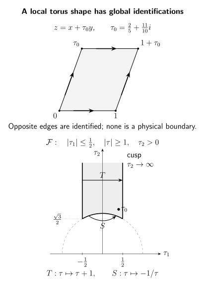
The lattice example uses $\tau_0=2/5+11i/10$. The upper-half-plane plot has equal real and imaginary scales and the quantitative boundary $|\tau|=1$. Lattice and modular-region edges represent identifications, not physical boundaries. The cusp $\tau_2\to\infty$ is a degenerating long-cylinder limit; the finite drawing truncates it.

There is one complex metric modulus on the unpunctured torus and one complex conformal Killing vector, the constant translation. There is also one holomorphic quadratic differential, the constant multiple of $dz^2$. Thus the ghost index is zero although both $b$ and $c$ have zero modes. The unstable pair $(g,n)=(1,0)$ is not covered by $K=3g-3+n$: inserting zero for its number of metric moduli would be incorrect. The vacuum calculation treats the translation volume, its ghost zero modes and the shape antighost insertion separately.

With at least one marked point, use translations to fix one position. The remaining $n-1$ relative positions plus $\tau$ give $n$ complex moduli, in agreement with the stable formula. Converting all movable punctures to integrated vertices leaves one $U$, one shape antighost pair and $n-1$ integrated matter vertices.

The real hyperbolic area form

$$\frac{d\tau_1\,d\tau_2}{\tau_2^2}$$

is modular invariant, as the last exercise verifies. It describes the geometry of the quotient; the full string integrand also includes matter and ghost determinants and zero-mode factors. A finite geometric area does not imply a finite vacuum amplitude. In particular, the bosonic tachyon causes infrared growth at the cusp, where the worldsheet develops a long propagation cylinder. This limitation is visible in the partition function analyzed by Tong, section 6.4.2.

What the gauge-fixed expression establishes

Gauge fixing removes redundant metric directions, retains true moduli, and associates each retained tangent with an antighost insertion. Residual conformal Killing vectors require their own treatment. Position antighosts explain the equivalence between fixed ghost-dressed vertices and integrated matter vertices.

These are local geometric and algebraic statements. A complete amplitude must also obey the quantum consistency conditions, transform correctly between moduli charts, include automorphism factors, and control degeneration boundaries. BRST symmetry arises from the gauge-fixed theory; the Weyl anomaly obstructs its quantum consistency rather than creating that symmetry. The next page derives this connection.

Exercises

Exercise 1. The gauge operator on a flat torus

On the flat unit torus let $v_a=u_a e^{ik\cdot x}$ with $k=2\pi(n_1,n_2)$, $n_a\in\mathbb Z$. Compute $P_1v$, its norm with the tensor inner product above, and $P_1^\dagger P_1v$. Determine the kernel and cokernel for $k=0$ and $k\ne0$.

Solution

The independent tensor components are

$$(P_1v)_{11}=i(k_1u_1-k_2u_2)e^{ik\cdot x},\qquad (P_1v)_{12}=i(k_1u_2+k_2u_1)e^{ik\cdot x},$$

and $(P_1v)_{22}=-(P_1v)_{11}$. Both off-diagonal entries contribute to the norm, so

$$\|P_1v\|_2^2 =2\bigl(|k_1u_1-k_2u_2|^2+|k_1u_2+k_2u_1|^2\bigr) =2|k|^2|u|^2.$$

The cross terms cancel for complex $u$ as well as real $u$. Direct differentiation gives

$$(P_1^\dagger P_1v)_b =-2\partial^a(\partial_av_b+\partial_bv_a-\delta_{ab}\partial\cdot v) =-2\Delta v_b=2|k|^2v_b.$$

For $k\ne0$ this map is injective. Both the vector space and the trace-free tensor space have two complex Fourier components, so it is also onto; there is no cokernel in this Fourier sector. At $k=0$, all constant vectors are in the kernel and all constant trace-free tensors are in the cokernel. For real fields these are two real translations and two real shape deformations, respectively. The overall trace is the separate Weyl direction.

Exercise 2. A complementary determinant

Take the reduced gauge columns and complementary columns

$$A_1=(1,1,0,0)^{\mathsf T},\quad A_2=(0,2,1,0)^{\mathsf T},\quad \mu_1=e_3,\quad\mu_2=e_4.$$

Evaluate their determinant through a Grassmann integral. Show how it changes under $\mu\mapsto\mu+AR$ and under $\mu\mapsto\mu J$. Explain the corresponding change of moduli coordinates.

Solution

The extended matrix is lower block-triangular with determinant $2$. In the exponential

$$e^{-(b_1+b_2)c_1-(2b_2+b_3)c_2},$$

the term containing both $c_1,c_2$, multiplied by $b_3b_4$, is the only one that can saturate all six variables. Terms containing a repeated $b_3$ vanish. The remaining coefficient, with the oriented Berezin measure of the main text, is $2$.

Adding $AR$ to the two last columns adds combinations of the first two columns, so the determinant is unchanged. This is the finite counterpart of changing a modulus representative by a gauge variation. Replacing the last columns by $\mu J$ multiplies the determinant by $\det J$.

If old coordinates obey $t=Jt'$ locally, then $\partial h/\partial t'=\mu J$ while $dt^1\wedge dt^2=(\det J)dt'^1\wedge dt'^2$. Thus the insertion product transforms with precisely the Jacobian needed when the old density is expressed in the new coordinates. For positive real measures the corresponding absolute Jacobian is used. Changing the tangent columns while leaving the coordinate density unchanged would describe a different expression.

Exercise 3. A complex four-puncture modulus

Fix three labeled points at $z_1=0$, $z_3=1$, $z_4=i$, and put $z_2=(1+i)/2$. Construct the Möbius map taking $z_1,z_3,z_4$ to $0,1,\infty$, calculate the remaining coordinate $x$, and check the integrated weight-(1,1) density locally. Which collisions are at $x=0,1,\infty$?

Solution

For general distinct fixed points the map is

$$f(z)=\frac{(z-z_1)(z_3-z_4)}{(z-z_4)(z_3-z_1)}.$$

Here $f(z)=(1-i)z/(z-i)$, and substitution gives $x=f(z_2)=1+i$. This configuration is not restricted to a real cross-ratio. Since

$$f'(z)=\frac{-(1+i)}{(z-i)^2},\qquad f'(z_2)=2-2i,$$

the local area Jacobian is $|f'(z_2)|^2=8$. The passive matter primary transforms as $V'(x)=V(z_2)/8$, so $d^2x\,V'(x)=d^2z_2\,V(z_2)$. The three fixed dressed operators are scalars; an insertion at infinity is defined by its local inverse coordinate or the corresponding primary limit.

The limits $z_2\to z_1,z_3,z_4$ give $x\to0,1,\infty$, respectively. These are degeneration limits, excluded from the interior of the four-punctured moduli space. Their singularities are physical factorization questions, not removable coordinate Jacobians.

Exercise 4. A puncture tangent as a contour

Let $\rho$ be a smooth cutoff equal to one near $q$ and zero outside a slightly larger disk. Use the representative $\mu_q=-\bar\partial\rho$ for translating the local coordinate $\zeta=z-q$. Show that its normalized $b$ pairing is $b_{-1}^{(q)}$. Then compute the ordered and reversed two-chirality actions on $U=c\widetilde cV$, and explain the fate of the position integral.

Solution

The derivative of $\rho$ is supported in an annulus where $b$ is holomorphic inside a correlator with no other insertion there. With the doubled complex measure, Stokes’ theorem gives

$$\int_{\rm annulus}d^2z\,\bar\partial(\rho b) =\frac1i\oint_{\partial\rm annulus}\rho b\,dz.$$

The outer boundary contributes zero; the inner boundary has clockwise orientation. Therefore

$$\frac1{2\pi}\int d^2z\,b(-\bar\partial\rho) =\frac1{2\pi i}\oint_{q,\,\mathrm{CCW}}b\,dz=b_{-1}^{(q)}.$$

The minus sign in $\mu_q$ corresponds to the coordinate change $\delta\zeta=-\delta q$. A different transition-coordinate convention changes both the tangent and its modulus orientation, not the physical density.

Using the odd residue actions as left derivatives,

$$b_{-1}(c\widetilde cV)=\widetilde cV,\qquad \widetilde b_{-1}(c\widetilde cV)=-cV.$$

Hence $\widetilde b_{-1}b_{-1}U=V$ and $b_{-1}\widetilde b_{-1}U=-V$. The antiholomorphic contour uses the physical-orientation minus sign stated in the main text.

The original modulus integral now integrates $V$ over $q$. Both antighost factors have already acted; they must not remain as additional factors. There is one position integral before and after descent. The annular argument assumes separated punctures; collisions can require contact terms or a continuation prescription.

Exercise 5. Ghost counting and the exceptional torus

For $(g,n)=(0,4),(1,2),(2,0)$, compare the all-unintegrated prescription with the usual mixed prescription. Explain why a naive application to $(1,0)$ misses a modulus, and why $n<3$ on the sphere does not mean a negative-dimensional space.

Solution

Count each chirality separately:

$$\begin{array}{c|c|c|c} (g,n)&K&\text{all fixed }(N_c,N_b)&N_c-N_b\\ \hline (0,4)&1&(4,1)&3\\ (1,2)&2&(2,2)&0\\ (2,0)&3&(0,3)&-3 \end{array}$$

On the sphere, descend one movable puncture: three $U$ remain, with one integrated matter vertex and no remaining shape antighost. On the torus, fix one point with translations and descend the other: one $U$ and one shape antighost remain, with one integrated matter vertex. On a genus-two vacuum surface there are no punctures or continuous conformal Killing vectors, and three complex shape moduli require three antighosts. Each result has degree $3-3g$.

For an unpunctured torus, $K_\Sigma$ is trivial. Both $H^0(K_\Sigma^2)$ and $H^0(T\Sigma)$ have complex dimension one. Their difference is zero, but the first space still supplies a shape modulus. The vanishing index is not a statement that each kernel vanishes. The translation volume and its ghost zero modes require the separate vacuum prescription.

On an unpunctured sphere there are three complex conformal Killing vectors and no smooth quadratic differentials. With fewer than three marked points, a continuous stabilizer remains after fixing the available positions. Subtracting three from $n$ is then an index count, not the dimension of an ordinary stable moduli space.

Exercise 6. Torus deformation and the area of the modular region

At fixed $x,y$ in $z=x+\tau y$, vary $\tau$ by $\delta\tau$. Derive the leading Beltrami coefficient relative to the old $z$ coordinate. Verify that $d\tau_1d\tau_2/\tau_2^2$ is invariant under a general real determinant-one Möbius transformation, and integrate it over $\mathcal F$. Does the finite answer imply a finite bosonic vacuum amplitude?

Solution

Since $y=(z-\bar z)/(\tau-\bar\tau)$, the changed complex coordinate satisfies

$$z'=z+\frac{\delta\tau}{2i\tau_2}(z-\bar z),\qquad dz'=\left(1+\frac{\delta\tau}{2i\tau_2}\right)dz -\frac{\delta\tau}{2i\tau_2}d\bar z.$$

Factoring the coefficient of $dz$ into the conformal scale gives the exact local Beltrami coefficient for this finite change,

$$\mu=\frac{-\delta\tau}{2i\tau_2+\delta\tau} =\frac{i\,\delta\tau}{2\tau_2}+O(|\delta\tau|^2).$$

Both the original and deformed tori must have positive imaginary part. This condition implies $|\mu|<1$, as required for an orientation-preserving complex structure. The change in the conformal scale is distinct from this trace-free deformation.

For $\tau'=(a\tau+b)/(c\tau+d)$ with real coefficients and $ad-bc=1$,

$$\frac{d\tau'}{d\tau}=\frac1{(c\tau+d)^2},\qquad \tau_2'=\frac{\tau_2}{|c\tau+d|^2}.$$

The two-dimensional real Jacobian is $|c\tau+d|^{-4}$, which cancels the transformation of $\tau_2^{-2}$. Thus the displayed hyperbolic area form is invariant. Its area on the standard region is

$$\int_{-1/2}^{1/2}d\tau_1 \int_{\sqrt{1-\tau_1^2}}^\infty\frac{d\tau_2}{\tau_2^2} =\int_{-1/2}^{1/2}\frac{d\tau_1}{\sqrt{1-\tau_1^2}} =\frac\pi3.$$

This is an explicitly real measure, so no extra factor from the worldsheet notation $d^2z$ enters. The answer is a geometric area, not a string partition function. Multiplication by an integrand that grows at the cusp can make the amplitude divergent; the bosonic tachyon is precisely such an obstruction.

References

• Polchinski, Joseph. “What Is String Theory?” Lectures at the 1994 Les Houches Summer School, in Fluctuating Geometries in Statistical Mechanics and Field Theory, edited by F. David, P. Ginsparg and J. Zinn-Justin, Elsevier, 1996, pp. 941–1104. arXiv:hep-th/9411028, section 2.7, especially equations (2.7.9)–(2.7.13).
• Tong, David. Lectures on String Theory. University of Cambridge lecture notes, 2009. arXiv:0908.0333, sections 5.1.1–5.1.3 and 6.4.1–6.4.2.