The Polyakov Action, Gauge Symmetry, and Virasoro Constraints

The Nambu–Goto action measures the area swept out by a string. Its square root makes the geometry transparent, but hides a useful simplification: in flat target spacetime, the classical equations can be written as free wave equations together with two constraints. The constraints are essential. Without them, the free fields describe many configurations that do not solve the string equations in the chosen gauge.

The Polyakov action exposes this structure by introducing an independent worldsheet metric. We will vary both the embedding and this metric, identify the gauge freedom, and explain why only $D-2$ local transverse degrees of freedom remain. This is a classical discussion; quantum anomalies and the physical-state conditions enter on later pages. We use the shared spacetime and worldsheet conventions, writing $T=T_{\rm F1}$ for the fundamental-string tension. The previous page develops the geometric action and its long-string approximation.

The auxiliary worldsheet metric

An embedding $X^\mu(\sigma)$ induces the metric

$$H_{ab}=G_{\mu\nu}(X)\partial_aX^\mu\partial_bX^\nu$$

on the worldsheet. It is determined by $X^\mu$; it cannot be varied independently. For a nondegenerate timelike worldsheet, the Nambu–Goto action is

$$S_{\rm NG}=-T\int d^2\sigma\sqrt{-\det H}.$$

Introduce a separate Lorentzian metric $\gamma_{ab}$ and define

$$S_{\rm P}[X,\gamma] =-\frac T2\int d^2\sigma\sqrt{-\gamma}\, \gamma^{ab}G_{\mu\nu}(X)\partial_aX^\mu\partial_bX^\nu, \qquad \gamma=\det\gamma_{ab}.$$

This metric has no derivatives in the action. Its equations will impose algebraic conditions on the embedding, rather than describe an additional propagating worldsheet graviton. In flat target space the action is quadratic in $X^\mu$ for a fixed $\gamma_{ab}$. A curved target produces an interacting nonlinear sigma model through the dependence of $G_{\mu\nu}$ on $X$.

The classical equivalence of the two actions follows by varying the auxiliary metric. The relevant identities are

$$\delta\sqrt{-\gamma} =-\frac12\sqrt{-\gamma}\,\gamma_{ab}\delta\gamma^{ab}, \qquad \delta(\gamma^{ab}H_{ab})=H_{ab}\delta\gamma^{ab}$$

when $X$ is held fixed. Thus

$$\delta_\gamma S_{\rm P} =-\frac T2\int d^2\sigma\sqrt{-\gamma} \left(H_{ab}-\frac12\gamma_{ab}\gamma^{cd}H_{cd}\right) \delta\gamma^{ab}.$$

Using the worldsheet constraint tensor defined in the overview, this variation gives

$$C_{ab}=H_{ab}-\frac12\gamma_{ab}\gamma^{cd}H_{cd}.$$

The metric equation is

$$C_{ab}=0 \quad\Longrightarrow\quad H_{ab}=\lambda\gamma_{ab}, \qquad \lambda=\frac12\gamma^{cd}H_{cd}.$$

For the ordinary positive-tension string we take the branch $\lambda>0$, so that the induced and auxiliary metrics assign the same timelike directions. On this branch,

$$\gamma^{ab}H_{ab}=2\lambda, \qquad \sqrt{-\det H}=\lambda\sqrt{-\gamma},$$

and substitution gives

$$S_{\rm P}\big|_{C_{ab}=0} =-T\int d^2\sigma\,\lambda\sqrt{-\gamma} =S_{\rm NG}.$$

The branch restriction is real information: the determinant identity alone gives $\sqrt{-\det H}=|\lambda|\sqrt{-\gamma}$. A negative $\lambda$ cannot be removed by a positive Weyl rescaling. This elimination argument also assumes $\det H\ne0$ in the interior. Collapsed strings and null portions of an embedding require separate care; a free open-string endpoint can become null even when the interior is timelike.

Diffeomorphisms and Weyl symmetry

Two gauge symmetries account for the apparent extra metric variables. Under a change of worldsheet coordinates $\sigma\mapsto\widetilde\sigma$, the embedding is a scalar and the metric is a tensor:

$$\widetilde X^\mu(\widetilde\sigma)=X^\mu(\sigma), \qquad \widetilde\gamma_{ab}(\widetilde\sigma) =\frac{\partial\sigma^c}{\partial\widetilde\sigma^a} \frac{\partial\sigma^d}{\partial\widetilde\sigma^b}\gamma_{cd}(\sigma).$$

The integrand is a scalar density, so the action is invariant. Such a transformation changes the description of the same embedded surface.

There is also the local Weyl transformation

$$\gamma_{ab}\longmapsto e^{2\omega(\sigma)}\gamma_{ab}, \qquad X^\mu\longmapsto X^\mu.$$

In two dimensions, $\sqrt{-\gamma}$ contributes $e^{2\omega}$ and $\gamma^{ab}$ contributes $e^{-2\omega}$; their product is unchanged. The trace of the metric variation therefore vanishes identically:

$$\gamma^{ab}C_{ab}=0.$$

Only two of the three symmetric metric equations are independent. The freedom in the positive factor $\lambda$ is precisely this Weyl redundancy.

Locally, coordinates can make a smooth two-dimensional Lorentzian metric conformally flat,

$$\gamma_{ab}=e^{2\omega}\eta_{ab}.$$

A Weyl transformation then removes $\omega$. This is conformal gauge. It is a gauge choice, not a consequence of $C_{ab}=0$. Globally, worldsheet topology, boundaries, and moduli can prevent one flat coordinate patch from covering the surface. None of the local argument removes those global data.

Quantum mechanically, the functional measure must also respect the proposed gauge symmetry. A Weyl anomaly can obstruct treating the conformal factor as redundant. The later critical-dimension and ghost calculations address that additional requirement; the classical argument alone places no restriction on $D$. Polyakov’s original paper discusses this distinction between classical geometry and the quantum measure in its path-integral formulation.

Why higher branes remain nonlinear

For comparison, the geometric embedding sector of a $p$-brane admits the auxiliary action

$$S_p=-\frac{\mathcal T_p}{2}\int d^{p+1}\sigma\sqrt{-\gamma} \left(\gamma^{ab}H_{ab}-(p-1)\right).$$

Here $\mathcal T_p$ denotes a general geometric tension; no D-brane charge formula is assumed. Write $K=\gamma^{ab}H_{ab}$. The metric equation and its trace are

$$H_{ab}-\frac12\gamma_{ab}\bigl(K-(p-1)\bigr)=0, \qquad (p-1)(p+1-K)=0.$$

For $p\ne1$, they give $K=p+1$ and $\gamma_{ab}=H_{ab}$, reproducing the geometric volume action. The auxiliary metric still has no propagating degrees of freedom: its equations are algebraic. What fails is the special two-dimensional simplification. The action is not Weyl invariant, and a general metric in dimension greater than two cannot be made flat by coordinate transformations. Eliminating the metric consequently restores the nonlinear embedding action. D-brane gauge fields, fermions, and charge couplings are additional fields and terms, beyond this geometric comparison.

Embedding equations and spatial boundaries

Varying $X^\mu$ in the full action gives

$$\frac1{\sqrt{-\gamma}}\partial_a \left(\sqrt{-\gamma}\gamma^{ab}\partial_bX^\mu\right) +\Gamma^\mu{}_{\nu\rho}(X) \gamma^{ab}\partial_aX^\nu\partial_bX^\rho=0.$$

The connection is that of the target metric $G_{\mu\nu}$. The first term differentiates the embedding on the worldsheet; the second makes the result transform covariantly in target space. For flat target spacetime it reduces to

$$\partial_a\left(\sqrt{-\gamma}\gamma^{ab}\partial_bX^\mu\right)=0.$$

Integration by parts also produces boundary terms. On a coordinate strip, with variations fixed at the initial and final times, the spatial contribution is unambiguously

$$\delta S_{\rm P}\big|_{\rm spatial} =-T\int d\tau\, \left[\sqrt{-\gamma}\gamma^{\sigma b} \partial_bX_\mu\,\delta X^\mu\right]_0^\pi.$$

In conformal gauge this becomes

$$\delta S_{\rm P}\big|_{\rm spatial} =-T\int d\tau\,[X'_\mu\delta X^\mu]_0^\pi.$$

For each target direction, the simplest choices are:

• Neumann: the endpoint variation is arbitrary and $X'^\mu=0$. The endpoint is free to move in that direction.
• Dirichlet: the endpoint position is prescribed, so $\delta X^\mu=0$. For a stationary endpoint value, $\dot X^\mu=0$ there as well.

A static D$p$-brane imposes Neumann conditions along its worldvolume, including target time, and Dirichlet conditions transverse to it. Background gauge fields or moving branes lead to more general conditions; they are not included here.

A closed string instead has periodic spatial data, so the contributions from the two sides of a cut cancel. A finite-time cylinder still has initial and final time slices, on which the variational problem fixes the appropriate data.

Conformal gauge leaves equations and constraints

In flat target spacetime, setting $\gamma_{ab}=\eta_{ab}$ gives

$$S_{\rm P}=\frac T2\int d\tau\,d\sigma \left(\dot X^2-X'^2\right), \qquad \ddot X^\mu-X''^\mu=0.$$

This action is easy to solve. However, substituting the gauge choice into the action before varying would discard the independent metric variations. Their equations must be retained:

$$C_{\tau\tau}=C_{\sigma\sigma} =\frac12(\dot X^2+X'^2)=0, \qquad C_{\tau\sigma}=\dot X\cdot X'=0.$$

The plus sign in $\dot X^2+X'^2$ is not a positivity contradiction: each square is a target-space Lorentzian contraction. For a timelike embedding, $\dot X^2$ can be negative.

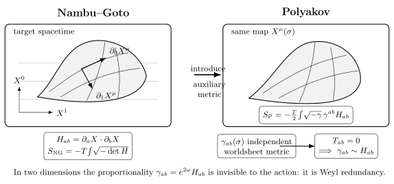
Vary the independent fields first. Eliminating the auxiliary metric on the nondegenerate positive branch recovers Nambu–Goto. Fixing conformal gauge instead gives free waves in flat target space, while preserving the metric constraints. The two operations have different purposes.

Using the worldsheet light-cone coordinates of the overview,

$$ds^2=-d\sigma^+d\sigma^-, \qquad \eta_{+-}=\eta_{-+}=-\frac12, \qquad \partial_+\partial_-X^\mu=0.$$

The local general solution is

$$X^\mu=X_L^\mu(\sigma^+)+X_R^\mu(\sigma^-).$$

Transforming the tensor components gives

$$\begin{aligned} C_{++}&=\frac14\left(C_{\tau\tau}+2C_{\tau\sigma}+C_{\sigma\sigma}\right) =(\partial_+X)^2,\\ C_{--}&=\frac14\left(C_{\tau\tau}-2C_{\tau\sigma}+C_{\sigma\sigma}\right) =(\partial_-X)^2,\\ C_{+-}&=\frac14\left(C_{\tau\tau}-C_{\sigma\sigma}\right)=0. \end{aligned}$$

Consequently the two independent metric equations are

$$(\partial_+X)^2=0, \qquad (\partial_-X)^2=0.$$

These are the classical Virasoro constraints. Each worldsheet null direction maps to a target-space null tangent. The surface need not be null: on a nondegenerate physical patch the two tangents are distinct, with $\partial_+X\cdot\partial_-X<0$. Their sum is timelike and their difference spacelike.

The wave equation also shows how constraints propagate:

$$\partial_-C_{++} =2\partial_+X\cdot\partial_-\partial_+X=0, \qquad \partial_+C_{--}=0.$$

Thus $C_{++}$ depends only on $\sigma^+$ and $C_{--}$ only on $\sigma^-$. Constraints imposed on initial data remain satisfied under the wave equation, provided the boundary conditions consistently join the incoming and outgoing data.

Residual symmetry and the open-string boundary

Conformal gauge still permits separate local reparametrizations of the null coordinates,

$$\widetilde\sigma^+=f^+(\sigma^+), \qquad \widetilde\sigma^-=f^-(\sigma^-).$$

For orientation-preserving functions with $f^{\pm\prime}>0$, the same metric written in the new coordinates is

$$ds^2 =-\frac{d\widetilde\sigma^+d\widetilde\sigma^-} {f^{+\prime}(\sigma^+)f^{-\prime}(\sigma^-)}.$$

The remaining factor is removed by a Weyl transformation. At a fixed coordinate argument, this passive transformation changes the component function by

$$\delta X^\mu =-\epsilon^+\partial_+X^\mu-\epsilon^-\partial_-X^\mu, \qquad f^\pm(u)=u+\epsilon^\pm(u).$$

The equivalent active pullback uses the opposite coordinate change and has $\delta X^\mu=+\epsilon^+\partial_+X^\mu+\epsilon^-\partial_-X^\mu$. This active form will be generated by canonical charges below. Stating which operation is meant fixes the apparent sign ambiguity.

In the bulk the two functions are independent. On the open-string strip they must preserve both boundaries. At $\sigma=0$ one has $\sigma^+=\sigma^-=\tau$, so boundary preservation requires

$$f^+(\tau)=f^-(\tau).$$

At $\sigma=\pi$, preservation of the coordinate width gives

$$f^+(\tau+\pi)-f^-(\tau-\pi)=2\pi.$$

Therefore $f^+=f^-=f$, with $f(u+2\pi)=f(u)+2\pi$. Infinitesimally, there is one independent function,

$$\epsilon^+(u)=\epsilon^-(u)=\epsilon(u), \qquad \epsilon(u+2\pi)=\epsilon(u).$$

Boundary conditions similarly relate the two chiral parts of the embedding. Neumann gives $\partial_+X=\partial_-X$ at the boundary; stationary Dirichlet gives $\partial_+X=-\partial_-X$ in that direction. In either case, squaring gives

$$C_{++}=C_{--} \quad\text{at each spatial boundary}.$$

Equivalently, the worldsheet energy flux, proportional to $C_{\tau\sigma}=C_{++}-C_{--}$, vanishes. This gluing explains why the open string has one set of Virasoro modes, while a closed string has two chiral sets, subject to their global periodicity conditions.

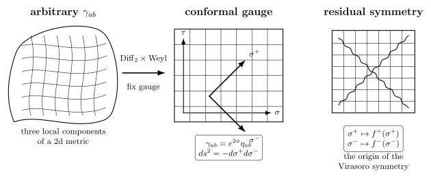
The strip has $0\leq\sigma\leq\pi$, with increasing $\tau$ upward. Both null directions are future-directed; reflection at a stationary boundary relates the two chiral sectors. A round trip takes worldsheet time $2\pi$, matching the periodicity of the residual infinitesimal reparametrization. Coordinate lengths are dimensionless, not target-space distances.

Canonical constraints and transverse motion

The canonical momentum in conformal gauge is $\Pi_\mu=T\dot X_\mu$. The two constraints can be written

$$\mathcal H_\perp =\frac1{2T}\left(\Pi^2+T^2X'^2\right)=0, \qquad \mathcal H_\parallel=\Pi\cdot X'=0.$$

They generate worldsheet deformations normal and tangential to a spatial slice. On a regular phase-space patch, they are first-class constraints: their Poisson brackets close on the constraints themselves. Each removes one phase-space variable through its equation and one through its associated gauge equivalence. Starting with the $2D$ local variables $(X^\mu,\Pi_\mu)$ gives

$$2D-2\times2=2(D-2)$$

physical phase-space dimensions per spatial point. This is $D-2$ local configuration degrees of freedom. One must not separately subtract the same gauge redundancy again after imposing these constraints.

A direct light-cone solution makes the count concrete; a complementary development appears in Tong’s lectures, section 2.2. Introduce target-space light-cone coordinates

$$X^\pm=\frac{X^0\pm X^{D-1}}{\sqrt2}, \qquad dX^2=-2dX^+dX^-+\sum_{i=1}^{D-2}(dX^i)^2.$$

These $X^\pm$ are target coordinates, whereas $\sigma^\pm$ label worldsheet directions. In a patch where the residual transformations can make $X^+$ a monotone clock, choose

$$X^+=x^++v^+\tau, \qquad v^+>0.$$

For an open string, this requires that the chosen target light-cone directions are compatible with its boundary conditions, for example Neumann conditions on both $X^0$ and $X^{D-1}$. The constraints then solve for the remaining longitudinal derivatives:

$$\partial_\pm X^- =\frac{\sum_i(\partial_\pm X^i)^2}{v^+}.$$

The $D-2$ transverse fields obey the wave equation freely; $X^-$ is reconstructed from them, up to zero-mode data and global consistency conditions. For a closed string, periodicity of the reconstruction will become the level-matching condition. The existence of this gauge is an assumption about the patch or solution, not a license to discard arbitrary zero modes.

The timelike field $X^0$ in the covariant action has a wrong-sign kinetic term. The classical constraints and gauge identifications explain why it is not an independent physical oscillator. Establishing a positive-norm quantum physical Hilbert space additionally requires the appropriate quantum constraints and anomaly cancellation; classical counting is not a no-ghost theorem.

From constraint densities to Virasoro generators

The chiral constraint densities with canonical normalization are

$$\mathcal C_\pm =\frac12(\mathcal H_\perp\pm\mathcal H_\parallel) =\frac1{4T}(\Pi\pm TX')^2 =T(\partial_\pm X)^2.$$

With $\{X^\mu(\sigma),\Pi_\nu(\sigma')\}=\delta^\mu{}_\nu\delta(\sigma-\sigma')$, define the smeared charges $\mathcal C_\pm[f]=\int d\sigma\,f(\sigma)\mathcal C_\pm(\sigma)$. For periodic fields on a closed string,

$$\begin{aligned} \{\mathcal C_\pm[f],\mathcal C_\pm[g]\} &=\pm\mathcal C_\pm[fg'-f'g],\\ \{\mathcal C_+[f],\mathcal C_-[g]\}&=0. \end{aligned}$$

The bracket closes, as required for first-class constraints. Its action on $X$ is

$$\{X^\mu,\mathcal C_+[f]+\mathcal C_-[g]\} =f\partial_+X^\mu+g\partial_-X^\mu.$$

These are the active residual transformations. For the closed string, at $\tau=0$ define

$$L_n=\int_0^{2\pi}d\sigma\,e^{in\sigma}\mathcal C_+, \qquad \widetilde L_n=\int_0^{2\pi}d\sigma\,e^{-in\sigma}\mathcal C_-.$$

The opposite Fourier signs compensate for the opposite orientations of the two chiral directions. The resulting brackets are

$$\begin{aligned} i\{L_m,L_n\}&=(m-n)L_{m+n},\\ i\{\widetilde L_m,\widetilde L_n\}&=(m-n)\widetilde L_{m+n},\\ \{L_m,\widetilde L_n\}&=0. \end{aligned}$$

At a different time, multiplying the corresponding integrals by $e^{in\tau}$ gives the same conserved modes. The constraints require all these classical modes to vanish. This is the centerless Virasoro algebra, also called the Witt algebra; quantization introduces normal ordering and can produce a central term. The current-bracket derivation is worked out in Exercise 4. Open-string modes use the boundary gluing above, rather than two independent periodic currents.

Target-space charges and boundary forces

Worldsheet constraints should not be confused with vanishing target-space energy. In flat target spacetime, translations and Lorentz transformations give the charges

$$P^\mu=T\int d\sigma\,\dot X^\mu, \qquad J^{\mu\nu}=T\int d\sigma \left(X^\mu\dot X^\nu-X^\nu\dot X^\mu\right).$$

Using the wave equation and integrating by parts on an open strip gives

$$\frac{dP^\mu}{d\tau}=T[X'^\mu]_0^\pi, \qquad \frac{dJ^{\mu\nu}}{d\tau} =T[X^\mu X'^\nu-X^\nu X'^\mu]_0^\pi.$$

Periodic data cancel these fluxes for a closed string. Pure Neumann boundary conditions cancel them for an unrestricted open string. Fixed Dirichlet boundaries can exert forces and torques, so the string alone need not conserve all of these charges. A static planar D-brane preserves translations along its worldvolume, and the corresponding string momenta are conserved; transverse translations are broken by fixing the brane position. If the brane is allowed to recoil, momentum conservation concerns the combined system.

This also separates two notions of energy. The conformal-gauge worldsheet Hamiltonian is the integral of $\mathcal H_\perp$ and vanishes on classical constrained configurations. The target-space energy is $P^0$, which need not vanish. The next page uses these charges for rotating strings and then quantizes their normal modes.

Exercises

Exercise 1: Eliminating the auxiliary metric for a higher brane

For the auxiliary $p$-brane action above, derive the metric equation, solve it for $p\ne1$, and verify the geometric action after substitution. Check explicitly why the action is Weyl invariant only for $p=1$. Does failure of Weyl invariance imply propagating metric excitations?

Solution

Let $d=p+1$ and $K=\gamma^{ab}H_{ab}$. Varying the inverse metric gives

$$\delta_\gamma S_p=-\frac{\mathcal T_p}{2}\int d^d\sigma\sqrt{-\gamma} \left[H_{ab}-\frac12\gamma_{ab}(K-(d-2))\right]\delta\gamma^{ab}.$$

The trace of the equation is

$$K-\frac d2(K-(d-2))=0 \quad\Longrightarrow\quad (d-2)(d-K)=0.$$

For $d\ne2$, this gives $K=d$ and then $H_{ab}=\gamma_{ab}$. Therefore

$$S_p=-\frac{\mathcal T_p}{2}\int d^d\sigma\sqrt{-\det H} \,[d-(d-2)] =-\mathcal T_p\int d^d\sigma\sqrt{-\det H}.$$

Under $\gamma_{ab}\mapsto e^{2\omega}\gamma_{ab}$, the $K$ term gains $e^{(d-2)\omega}$, whereas the constant term gains $e^{d\omega}$. These cannot cancel for arbitrary local $\omega$. For $d=2$ the constant vanishes and the kinetic term is invariant. For $d\ne2$ the metric remains auxiliary because there are no $\partial\gamma$ terms. The equations algebraically determine it; absence of Weyl invariance is not a metric kinetic term.

Exercise 2: A wave is not automatically a constrained string

Consider the strip embedding

$$X^0=a\tau, \qquad X^1=b\sigma, \qquad X^{\mu>1}=0, \qquad a,b>0.$$

Impose Neumann conditions on $X^0$ and fixed Dirichlet values $X^1(0)=0$, $X^1(\pi)=b\pi$. Show that the wave equation and boundary conditions hold for every $a,b$, but the metric constraints in conformal gauge do not. In the allowed case compute $P^0$ and the physical string length. Explain why the same planar surface with $a\ne b$ can still be described by the Nambu–Goto action.

Solution

All second derivatives vanish, as does $X'^0$. The induced metric and conformal-gauge constraint components are

$$H_{ab}=\operatorname{diag}(-a^2,b^2), \qquad C_{\tau\sigma}=0, \qquad C_{\tau\tau}=C_{\sigma\sigma}=\frac12(-a^2+b^2).$$

Thus conformal gauge requires $a=b$. The target length is $L=b\pi$, and

$$P^0=T\int_0^\pi a\,d\sigma=\pi Ta=TL.$$

For $a\ne b$, this is still a flat timelike surface and a solution of the Nambu–Goto embedding equations. Its equivalent Polyakov description may take $\gamma_{ab}=H_{ab}$; it does not take $\gamma_{ab}=\eta_{ab}$ in these same coordinates. A change of time coordinate $\widetilde\tau=(a/b)\tau$ brings the induced metric to $b^2\eta_{ab}$ while preserving the strip width. The example distinguishes an embedded surface from a surface and an incompatible gauge-fixed auxiliary metric.

Exercise 3: A residual transformation on the strip

Find the conditions on the infinitesimal functions $\epsilon^\pm$ imposed by both strip boundaries. For $\epsilon(u)=\sin(nu)$ with integer $n\ne0$, find the coordinate shifts $\delta\tau$ and $\delta\sigma$. Show that the normal shift vanishes at each boundary and explain why a generic nonperiodic function fails.

Solution

For the passive coordinate shift, the normal component is

$$\delta\sigma=\frac12\left[\epsilon^+(\tau+\sigma)-\epsilon^-(\tau-\sigma)\right].$$

At $\sigma=0$ this vanishes for every $\tau$ only if $\epsilon^+(u)=\epsilon^-(u)=\epsilon(u)$. At $\sigma=\pi$ it requires $\epsilon(\tau+\pi)=\epsilon(\tau-\pi)$, hence $2\pi$ periodicity. For the sine mode,

$$\delta\tau=\sin(n\tau)\cos(n\sigma), \qquad \delta\sigma=\cos(n\tau)\sin(n\sigma).$$

The latter vanishes at $0$ and $\pi$ because $n$ is integer. A small transformation with a nonperiodic $\epsilon$ can preserve the left boundary while moving the right one; it therefore fails to preserve the specified coordinate strip. Multiplying the sine mode by a sufficiently small real amplitude also ensures that its finite continuation preserves orientation.

Exercise 4: The classical Virasoro brackets

For a closed string, introduce $J_\pm^\mu=\Pi^\mu\pm TX'^\mu$. Derive their equal-time Poisson brackets and use them to obtain the brackets of $\mathcal C_\pm=J_\pm^2/(4T)$. Recover the algebra of the modes defined above. Keep the sign difference between the two chiralities explicit.

Solution

The canonical brackets imply

$$\begin{aligned} \{\Pi^\mu(\sigma),X'^\nu(\sigma')\} &=\eta^{\mu\nu}\partial_\sigma\delta(\sigma-\sigma'),\\ \{X'^\mu(\sigma),\Pi^\nu(\sigma')\} &=\eta^{\mu\nu}\partial_\sigma\delta(\sigma-\sigma'). \end{aligned}$$

Here $\delta$ is the periodic delta distribution. Hence

$$\{J_\pm^\mu(\sigma),J_\pm^\nu(\sigma')\} =\pm2T\eta^{\mu\nu}\partial_\sigma\delta(\sigma-\sigma'), \qquad \{J_+^\mu,J_-^\nu\}=0.$$

Applying the product rule to the squared currents gives

$$\{\mathcal C_\pm(\sigma),\mathcal C_\pm(\sigma')\} =\pm\frac{J_\pm(\sigma)\cdot J_\pm(\sigma')}{2T} \partial_\sigma\delta(\sigma-\sigma').$$

As a distribution this is equivalently

$$\{\mathcal C_\pm(\sigma),\mathcal C_\pm(\sigma')\} =\pm[\mathcal C_\pm(\sigma)+\mathcal C_\pm(\sigma')] \partial_\sigma\delta(\sigma-\sigma').$$

To check the replacement, the difference of the coefficients is proportional to $(J_\pm(\sigma)-J_\pm(\sigma'))^2$, which has a double zero at $\sigma=\sigma'$ and therefore annihilates $\delta'$. Smearing and integrating by parts, with no endpoint term on the circle, yields

$$\{\mathcal C_\pm[f],\mathcal C_\pm[g]\} =\pm\int d\sigma\,\mathcal C_\pm(fg'-f'g).$$

For the plus sector, choose $f=e^{im\sigma}$ and $g=e^{in\sigma}$. The factor $fg'-f'g=i(n-m)e^{i(m+n)\sigma}$ gives $i\{L_m,L_n\}=(m-n)L_{m+n}$. For the minus sector, both Fourier exponents have the opposite sign; this compensates the minus sign in the current bracket and yields the same mode algebra. Mixed brackets vanish. There is no classical central term: every term is proportional to a constraint density.

Exercise 5: Momentum exchange with fixed endpoints

Start with a straight string $X^0=b\tau$, $X^1=b\sigma$, and add a small transverse displacement

$$Y(\tau,\sigma)=A\sin\sigma\cos\tau, \qquad |A|\ll b.$$

Treat it as a linearized fluctuation with fixed endpoints. Compute its transverse momentum and its rate of change with respect to target time $t=b\tau$. Verify the boundary-force formula. Why is a time-dependent transverse momentum compatible with Dirichlet conditions?

Solution

The fluctuation obeys the wave equation and vanishes at both endpoints. Its contribution to the constraints begins at order $A^2$, so the stated embedding is consistent through linear order; longitudinal corrections would be needed beyond that order. The transverse momentum is

$$P_Y=T\int_0^\pi d\sigma\,\dot Y =-2TA\sin\tau.$$

Thus, to this order,

$$\frac{dP_Y}{dt} =-\frac{2TA}{b}\cos\tau.$$

The boundary gradients are $Y'(0)=A\cos\tau$ and $Y'(\pi)=-A\cos\tau$. Dividing the conformal-time flux by $dt/d\tau=b$ gives

$$\frac Tb[Y']_0^\pi =-\frac{2TA}{b}\cos\tau,$$

in agreement. When the string bows toward positive $Y$, both supports exert a restoring transverse force on it. Dirichlet conditions fix endpoint positions, not the forces applied there. The string exchanges transverse momentum with the supports, while its endpoint velocities vanish and the supports do no work. Energy conservation and conservation of every momentum component are different statements.

Exercise 6: Reconstructing a longitudinal coordinate

In a local target light-cone gauge $X^+=x^++v^+\tau$, choose one transverse standing wave on the open strip,

$$X^1=A\cos(n\sigma)\cos(n\tau), \qquad n=1,2,\ldots,$$

with the other transverse coordinates constant. Assume Neumann conditions for the target light-cone directions. Reconstruct $X^-$ from the two constraints, verify its wave equation and Neumann conditions, and identify its average linear growth in $\tau$. This exercise concerns a classical solution; no quantum intercept is present.

Solution

Decompose the standing wave into chiral parts:

$$X^1=\frac A2\left[\cos(n\sigma^+)+\cos(n\sigma^-)\right], \qquad \partial_\pm X^1=-\frac{An}{2}\sin(n\sigma^\pm).$$

The constraints give

$$\partial_\pm X^- =\frac{A^2n^2}{4v^+}\sin^2(n\sigma^\pm) =\frac{A^2n^2}{8v^+}\left[1-\cos(2n\sigma^\pm)\right].$$

Integrating the two chiral functions independently yields

$$\begin{aligned} X^-={}&x^-+\frac{A^2n^2}{8v^+}(\sigma^++\sigma^-) -\frac{A^2n}{16v^+}\left[\sin(2n\sigma^+)+\sin(2n\sigma^-)\right]\\ ={}&x^-+\frac{A^2n^2}{4v^+}\tau -\frac{A^2n}{8v^+}\sin(2n\tau)\cos(2n\sigma). \end{aligned}$$

Each term is either linear or a product of equal-frequency sine and cosine functions, so $\ddot X^--X^{-\prime\prime}=0$. Its spatial derivative contains $\sin(2n\sigma)$ and vanishes at both endpoints. Averaging over a period removes the oscillatory term, giving $\langle\dot X^-\rangle=A^2n^2/(4v^+)$. The longitudinal motion is fixed by the transverse wave and the chosen $v^+$, rather than representing another freely specifiable oscillator. Points where the induced metric degenerates require the qualification discussed at the start of the page; the Polyakov equations themselves remain well-defined there.

References

• Polyakov, A. M. “Quantum geometry of bosonic strings.” Physics Letters B 103, no. 3 (1981): 207–210. doi:10.1016/0370-2693(81)90743-7. The original path-integral treatment distinguishes the classical auxiliary metric from the quantum conformal anomaly.
• Tong, David. String Theory. University of Cambridge Part III Mathematical Tripos lecture notes (2009), sections 1.3–1.4, 2.2, and 3. arXiv:0908.0333. A complementary treatment of the classical action, light-cone reduction, and open-string boundary conditions.