D-brane dynamics, tachyon condensation, and RR charges

A D-brane can move, support a gauge field, and carry spacetime charge. The Dirac–Born–Infeld (DBI) action combines its motion and gauge dynamics in one determinant; the Wess–Zumino (WZ) action specifies its Ramond–Ramond (RR) couplings. Together they explain how the open-string degrees of freedom found on the previous page become a theory of dynamical extended objects. An unstable brane requires additional tachyon degrees of freedom, and its disappearance is a separate question about the energy and charge of the vacuum.

The main calculations below concern a single BPS type II D-brane, its leading action in the string coupling, and slowly varying fields. The bosonic brane and unstable type II systems are distinguished when tachyons enter. Metric and matrix-field definitions follow the String I global conventions; the shared D-brane normalizations and RR potential basis fix the action coefficients and charge signs.

D-brane fields and induced geometry

A D$p$-brane has a $(p+1)$-dimensional worldvolume $\mathcal W_{p+1}$. Locally, choose static gauge $X^a=\xi^a$, with $a=0,\ldots,p$. The remaining embedding functions $X^i(\xi)$, $i=p+1,\ldots,9$, describe transverse motion. They are scalar fields under worldvolume coordinate changes, although they carry a transverse spacetime index.

The pullback of the string-frame metric is

$$g_{ab}=P[G^{\rm S}]_{ab} =G^{\rm S}_{MN}(X)\,\partial_aX^M\partial_bX^N.$$

In flat space this becomes

$$g_{ab}=\eta_{ab}+\partial_aX^i\partial_bX^i.$$

The second term is geometric: a slope or velocity changes the length or proper time measured on the brane. It is not an extra bulk metric perturbation. Static gauge is a local description of an embedding that can be expressed as a graph.

The massless bosons of an oriented open string supply a worldvolume gauge field $A_a$ and the transverse scalars. T-duality fixes their relative normalization:

$$X^i=y_0^i+2\pi\alpha'\Phi^i.$$

Thus $[X^i]=L$, whereas $[A_a]=[\Phi^i]=L^{-1}$ when $[\xi^a]=L$. For $p\geq1$, the gauge field has $p-1$ physical polarizations and the embedding has $9-p$ transverse fluctuations: there are eight bosonic on-shell degrees of freedom in total. For a D0-brane, $A_0$ instead imposes a constraint and the nine transverse positions are worldline variables; there is no massless worldvolume particle little group to which the preceding polarization count applies. Fermions complete the supersymmetric theory, but will not be needed for the following bosonic calculations.

For $N$ coincident branes the fields become Hermitian $N\times N$ matrices. Commuting diagonal scalar expectation values describe separated positions. General noncommuting matrices do not define $N$ simultaneous classical positions.

The DBI determinant from T-duality

Why should the gauge field and the induced metric enter the same determinant? Start with an Abelian gauge field on a higher-dimensional flat brane, independent of a set of compact worldvolume coordinates $y^i$. Write $q=2\pi\alpha'$ as an abbreviation in this derivation. Then

$$F_{ai}=\partial_a A_i, \qquad F_{ia}=-\partial_a A_i, \qquad F_{ij}=0.$$

The matrix in its Born–Infeld action has the block form

$$M= \begin{pmatrix} \eta_{ab}+qF_{ab}&q\partial_aA_j\\ -q\partial_bA_i&\delta_{ij} \end{pmatrix}.$$

Multiplying on the left by a block triangular matrix of determinant one gives the identity

$$\begin{pmatrix}1&-B\\0&1\end{pmatrix} \begin{pmatrix}A&B\\C&1\end{pmatrix} = \begin{pmatrix}A-BC&0\\C&1\end{pmatrix}, \qquad \det M=\det(A-BC).$$

Here $C=-B^{\mathsf T}$, so the correction has a plus sign. With the dual coordinates $X^i=qA_i$,

$$\det M =\det\!\left(\eta_{ab}+qF_{ab} +q^2\partial_aA_i\partial_bA_i\right) =\det(g_{ab}+qF_{ab}).$$

The former gauge components have become the induced metric of a moving lower-dimensional brane. This is the determinant form of the open-string T-duality relation.

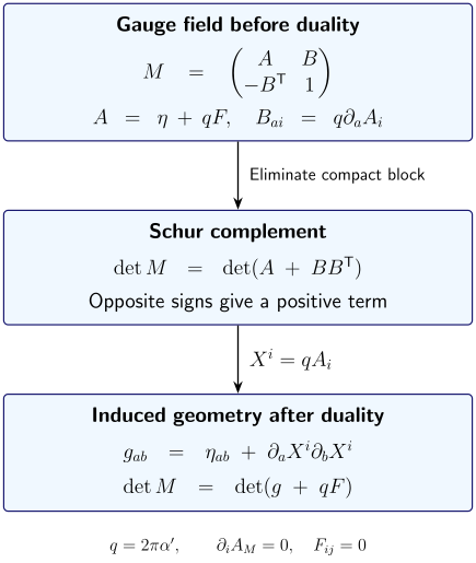
For fields independent of the compact directions and $F_{ij}=0$, the Schur complement converts $A_i$ to the transverse position $X^i=2\pi\alpha'A_i$. The minus sign in the lower off-diagonal block is essential: it produces $+\partial_aX^i\partial_bX^i$. This diagram represents an algebraic identity, not a spacetime trajectory.

The overall coefficient also agrees. For one wrapped circle of radius $R$, T-duality sends $g_s$ to $g_s'=g_s\sqrt{\alpha'}/R$. The physical tensions in the respective theories obey

$$2\pi R\,T_{p+1}(g_s)=T_p(g_s').$$

Thus integrating the higher-dimensional action over the circle gives the lower-dimensional action with its correct tension, not only the correct determinant.

This argument assumes the Born–Infeld dependence on a constant Abelian field strength. Its string-theory justification comes from the disk calculation and its derivative expansion; see Tseytlin, sections 2–3. T-duality then explains the geometric completion. It does not establish all higher-derivative terms or a complete non-Abelian determinant prescription.

Gauge invariance and the small-field limit

In a slowly varying background, the single-brane action is

$$S_{\rm DBI} =-\mu_p\int_{\mathcal W_{p+1}}d^{p+1}\xi\, e^{-\Phi}\sqrt{-\det(g_{ab}+\mathcal B_{ab})}, \qquad \mathcal B=P[B_2]+2\pi\alpha'F.$$

Here $\Phi$ is the total dilaton. Consequently $\mu_pe^{-\Phi}=T_pe^{-\phi}$ in the global normalization. At constant asymptotic dilaton the prefactor is the physical tension $T_p$. Its $g_s^{-1}$ scaling is characteristic of a disk contribution: the brane becomes heavy in the weakly coupled closed-string description.

The two-form combination follows from gauge invariance. Under $B_2\mapsto B_2+d\Lambda_1$, the boundary gauge field changes by $A\mapsto A-P[\Lambda_1]/(2\pi\alpha')$. Since pullback commutes with exterior differentiation,

$$\delta\mathcal B =P[d\Lambda_1]-dP[\Lambda_1]=0.$$

This is also the cancellation between the gauge variation of the worldsheet $B$ coupling and its boundary coupling. A bare $F$ term would miss that cancellation in a nonzero $B$ background.

Set $B=0$, take flat space and constant dilaton, and let $q=2\pi\alpha'$. The matrix identity

$$\sqrt{\det(1+K)} =\exp\!\left[\frac12\operatorname{tr}\log(1+K)\right]$$

organizes the expansion. For $K^a{}_b=qF^a{}_b$, antisymmetry implies $\operatorname{tr}K=0$ and

$$\operatorname{tr}K^2=-q^2F_{ab}F^{ab}.$$

The scalar correction $\partial_aX^i\partial_bX^i$ is already quadratic in the fluctuations. Retaining quadratic terms gives

$$\begin{aligned} S_{\rm DBI}=-T_p\int d^{p+1}\xi\, \left[1+\frac12\partial_aX^i\partial^aX^i +\frac{q^2}{4}F_{ab}F^{ab}+\cdots\right]. \end{aligned}$$

The mostly-plus metric makes the scalar time-derivative term in the Lagrangian positive. With $X^i-y_0^i=q\Phi^i$, the quadratic action is

$$S^{(2)}=-\frac1{g_{\rm A}^2}\int d^{p+1}\xi\, \left(\frac14F_{ab}F^{ab} +\frac12\partial_a\Phi^i\partial^a\Phi^i\right),$$

where

$$\frac1{g_{\rm A}^2}=T_p(2\pi\alpha')^2, \qquad g_{\rm A}^2=(2\pi)^{p-2}g_s(\alpha')^{(p-3)/2}.$$

The dimension $[g_{\rm A}^2]=L^{p-3}$ agrees with a gauge theory in $p+1$ dimensions. In particular, the D3 coupling is dimensionless.

For a stack, the disk sum replaces the single-brane expression by a fundamental matrix trace at leading order. Comparing $-\operatorname{tr}F^2/(4g_{\rm A}^2)$ with the globally defined $-\operatorname{tr}F^2/(2g_{\rm YM}^2)$ yields

$$g_{\rm YM}^2=2g_{\rm A}^2, \qquad p=3:\quad g_{\rm YM}^2=4\pi g_s.$$

The factor of two compares two specified actions and generator normalizations; changing the coupling alone would change the physics. Dimensional reduction of this leading matrix action also gives $D_a\Phi^i$ and a nonnegative static potential,

$$V=\frac1{4g_{\rm A}^2}\sum_{i,j} \operatorname{tr}\!\left( [\Phi^i,\Phi^j]^\dagger[\Phi^i,\Phi^j]\right).$$

For Hermitian scalars the commutator is anti-Hermitian. Thus this expression is equivalent to a minus sign times $\operatorname{tr}[\Phi^i,\Phi^j]^2$, and vanishes for commuting positions. It should not be confused with a claim that ordinary matrix ordering makes the entire Abelian DBI determinant exact.

DBI retains all powers of constant $F$ at the disk level while omitting derivative corrections. Small $qF$ is needed for the Maxwell truncation, but not for using the constant-field determinant. Slowly varying fields, small string-scale curvature and suppressed string loops are separate requirements. Near a critical electric field, large gradients or a tachyon instability, a low-order effective action needs additional scrutiny.

Relativistic motion and electric displacement

For a D0-brane at constant dilaton, $F$ has no two-form component and

$$S_{D0}=-T_0\int dt\,\sqrt{1-\dot{\mathbf X}^{2}}.$$

The rest mass is $T_0$; the expansion reproduces $T_0\dot{\mathbf X}^{2}/2$. The brane position has acquired the correct relativistic particle dynamics without adding a separate kinetic term.

For a D1-brane, put $\mathbf v=\partial_t\mathbf X$, $\mathbf u=\partial_x\mathbf X$ and $E=F_{tx}$. Directly taking the two-by-two determinant gives

$$-\det(g+qF) =(1-\mathbf v^2)(1+\mathbf u^2) +(\mathbf v\cdot\mathbf u)^2-q^2E^2.$$

Only for one transverse scalar, or parallel $\mathbf v$ and $\mathbf u$, does the quartic combination $-\mathbf v^2\mathbf u^2+(\mathbf v\cdot\mathbf u)^2$ cancel. The familiar square root $\sqrt{1+X'^2-\dot X^2}$ therefore has a definite domain of application.

For a flat, static D$p$-brane with one constant electric component and no magnetic field, the Lagrangian density reduces to

$$\mathcal L(E)=-T_p\sqrt{1-q^2E^2}.$$

The electric branch connected to the vacuum has $|qE|<1$. Its conjugate displacement and Hamiltonian density are

$$\mathcal D=\frac{\partial\mathcal L}{\partial E} =\frac{T_pq^2E}{\sqrt{1-q^2E^2}}, \qquad \mathcal H=\mathcal D E-\mathcal L =\sqrt{T_p^2+\left(\frac{\mathcal D}{q}\right)^2}.$$

Equivalently, defining dimensionless response variables $e=qE$ and $d=\mathcal D/(T_pq)$,

$$e=\frac{d}{\sqrt{1+d^2}}, \qquad \frac{\mathcal H}{T_p}=\sqrt{1+d^2}.$$

A finite displacement gives a finite energy and a subcritical field. Approaching $|e|=1$ requires $|d|\to\infty$ in this classical branch. The vanishing of the DBI square root at a prescribed critical field does not mean that the energy of the flux vanishes: energy is obtained by a Legendre transform. On a compact D1-brane, quantizing this displacement yields fundamental-string charge, as exercise 3 shows.

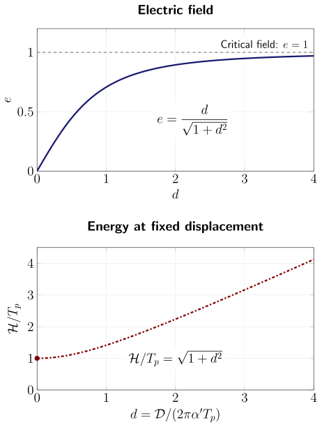
For a flat static brane with one constant electric field, $d=\mathcal D/(2\pi\alpha'T_p)$ determines $e=2\pi\alpha'E$ and the total energy density $\mathcal H/T_p$. The positive branch is plotted with exact dimensionless axes; negative $d$ follows by oddness of $e$ and evenness of the energy. The dashed line is the limiting field $e=1$, approached only at infinite displacement.

RR couplings and charge carried by flux

The DBI action couples the brane to the metric, dilaton and NS two-form. For a BPS type II brane, the leading RR coupling is

$$S_{\rm WZ} =\mu_p\int_{\mathcal W_{p+1}} \left.P\!\left[\sum_n C_n^{\rm WZ}\right] \wedge e^{\mathcal B}\right|_{p+1}.$$

The subscript selects the $(p+1)$-form component. The superscript identifies the shared WZ potential basis, which is required for this plus-exponential formula; it cannot be dropped while silently substituting differently defined bulk potentials. This is the Abelian coupling without curvature corrections. The more general action contains additional gravitational couplings, and matrix-valued scalars require further terms. Myers, equations (3)–(5) provides the relevant starting point.

The leading term $+\mu_p\int P[C_{p+1}^{\rm WZ}]$ defines a positive oriented D$p$ charge. An antibrane reverses this coupling but keeps the positive DBI tension. The numerical coefficient $\mu_p$ and the physical tension $T_p=\mu_p/g_s$ are not equal; the BPS relation compares charge and energy after the bulk field and supersymmetry algebra have been normalized consistently.

To see what the exponential does, consider a D2-brane wrapping a compact oriented surface $\Sigma_2$, with $B=0$. Its coupling contains

$$\mu_2\int C_1^{\rm WZ}\wedge 2\pi\alpha'F.$$

For a unit-charge line bundle,

$$\frac1{2\pi}\int_{\Sigma_2}F=n\in\mathbb Z.$$

Assuming $C_1^{\rm WZ}$ is pulled back along the remaining worldline, the integral reduces to

$$\mu_2(2\pi\alpha')(2\pi n)\int C_1^{\rm WZ} =n\mu_0\int C_1^{\rm WZ}.$$

There are $n$ units of D0 charge on the wrapped D2. The sign is the sign of the oriented flux. This is a charge statement obtained directly from the action; it does not require a picture of separated pointlike D0-branes. On a D4, the $F\wedge F/2$ term likewise produces D0 charge, and exercise 4 checks its coefficient and its energy cost.

The interpretation of D-branes as RR sources is a physical result of string theory, established through their couplings and exchange amplitudes; see Polchinski. A bosonic D-brane has no RR charge because the bosonic string has no RR sector. Its boundary condition and Born–Infeld gauge dynamics therefore do not imply the type II WZ action.

Tachyon condensation and the vacuum energy

An open-string tachyon is a fluctuation with negative mass squared about a particular brane configuration. The configuration is a stationary point with a downward direction in its potential, not a particle travelling faster than light. For a bosonic open string, $m^2=-1/\alpha'$; for the tachyon on a type II non-BPS brane or coincident brane–antibrane pair, $m^2=-1/(2\alpha')$.

Let $\mathcal T_{\rm u}$ be the tension of the entire unstable system, and choose the relative potential $V$ to vanish at the perturbative brane configuration. The total static energy density is then

$$U(t)=\mathcal T_{\rm u}+V(t), \qquad V(0)=0.$$

The tachyon-vacuum energy statement is

$$V(t_*)=-\mathcal T_{\rm u}, \qquad U(t_*)=0.$$

It is a statement about the energy difference between two stationary configurations. It must be supplemented by the absence of perturbative open-string excitations at the vacuum; changing a potential by a constant alone says nothing about that spectrum. The derivations and evidence from boundary conformal field theory and open string field theory are reviewed by Sen, sections 2–3. A controlled string-field-theory example is developed on the String II tachyon page.

The tension to be cancelled depends on the system:

Unstable system	Initial tension $\mathcal T_{\rm u}$	Tachyon and charge
One bosonic D25-brane	Its bosonic D25 tension	Real open tachyon; no RR sector
One type II non-BPS D$p$-brane	$\sqrt2\,T_p$	Real tachyon; no net ordinary BPS D$p$ charge
Coincident BPS D$p$–anti-D$p$ pair	$2T_p$	Complex bifundamental tachyon; net D$p$ charge zero

In the non-BPS row, $T_p$ denotes the BPS tension formula evaluated at $p$, even though a BPS brane of that dimension belongs to the other type II theory. The non-BPS parity is opposite to the BPS parity. In the pair row, the two equal tensions add, whereas the RR charges cancel.

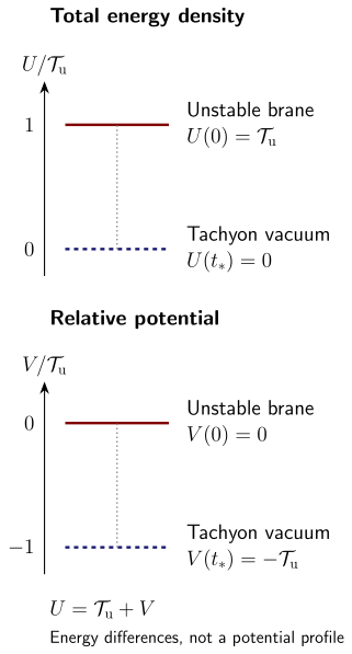
The two panels express the same energy difference in units of the full unstable-system tension $\mathcal T_{\rm u}$. Total energy decreases from $1$ to $0$ between the two configurations; the relative potential changes from $0$ to $-1$. The connecting marks compare stationary energy levels. They do not specify a potential as a function of the tachyon, or a real-time decay trajectory.

Several qualifications matter. The tachyon field coordinate and the shape of its off-shell potential depend on the description; the vacuum may occur at an infinite value of a chosen field coordinate. A double-well sketch does not determine an exact string potential. A spatially varying tachyon can leave a lower-dimensional charged defect, so homogeneous annihilation is not the only possible configuration. In a real decay, energy remains in fields, radiation or other excitations; the difference of static vacuum energies is not a violation of energy conservation. Finally, removing a bosonic open tachyon does not remove the closed-string tachyon of the bosonic background.

A BPS type II brane has no perturbative open tachyon. Its nonzero conserved RR charge prevents it from disappearing into the uncharged vacuum. Charge can instead be balanced by an antibrane or carried by other objects and flux. The stable-brane DBI action, which contains no tachyon field, cannot by itself derive these unstable-system potentials or their endpoints.

Electric and magnetic RR branes

The form degree gives a useful classification. An electric D$p$ source couples to $C_{p+1}^{\rm WZ}$. In a region with $B=0$ and no sources, its linearized field strength $\mathcal F_{p+2}=dC_{p+1}^{\rm WZ}$ has a dual of degree $8-p$. The dual potential has degree $7-p$, so its electric source has spatial dimension $6-p$:

$$\text{D0}\leftrightarrow\text{D6},\qquad \text{D1}\leftrightarrow\text{D5},\qquad \text{D2}\leftrightarrow\text{D4},\qquad \text{D3}\leftrightarrow\text{D3}.$$

These are the ordinary Lorentzian pairs with $0\leq p\leq6$. The form-degree argument fixes which branes are paired; it does not determine an oriented flux sign. That sign follows from the global democratic duality relation, including its degree-dependent factor and the Lorentzian Hodge star. In particular, writing $\mathcal F_{8-p}=*\mathcal F_{p+2}$ with a universal plus sign would be incorrect. The charge and Dirac-quantization page derives the oriented source equations.

The minimal positive charge magnitudes obey

$$2\kappa_{10,0}^2\mu_p\mu_{6-p}=2\pi,$$

where $\kappa_{10,0}=\kappa_{10}/g_s$ is the centrally defined coupling without the asymptotic string coupling. Exercise 6 verifies the normalization. This is the magnitude of the Dirac pairing; an antibrane changes a source sign. The IIB five-form is self-dual, so the D3 case uses a constrained self-dual field rather than two independent five-form fields.

Type II T-duality reflects one right-moving worldsheet fermion as well as its boson. It therefore flips the right Ramond chirality, exchanges IIA with IIB, and changes a wrapped D$p$ to D$(p-1)$ or a transverse D$p$ to D$(p+1)$. The compatible BPS pattern is:

Theory	Ordinary Lorentzian branes	Additional cases
IIA	D0, D2, D4, D6	D8 couples to a nine-form; its dual zero-form is the Romans mass
IIB	D1, D3, D5, D7	Euclidean D$(-1)$ instanton; space-filling D9 couples to a top-form potential

The D7 is related to the axion and its monodromy; its electric dual is a Euclidean D-instanton, rather than a negative-dimensional Lorentzian worldvolume. A D8 separates regions with different Romans mass. The ten-form potential coupled to a D9 has no propagating eleven-form field strength in ten dimensions; its charge is subject to the appropriate cancellation constraints. These cases cannot be obtained by extending the ordinary propagating-field pairing to fictitious Lorentzian D$(-2)$ or D$(-3)$ objects.

RR couplings under T-duality

The change of brane dimension also determines how RR potentials change degree. Consider a flat circle with physical coordinate $y\sim y+2\pi R$, a circle isometry, $B=0$ and vanishing worldvolume flux. Use the shared WZ basis and put the compact index last in the oriented worldvolume. For a D$p$ wrapped once on the circle, equality of the reduced WZ couplings requires

$$\mu_p(2\pi R)\,C^{\rm WZ}_{a_1\cdots a_p y} =\mu_{p-1}\,C^{{\rm WZ}\prime}_{a_1\cdots a_p}.$$

Since $\mu_p/\mu_{p-1}=1/(2\pi\ell_s)$, a component carrying the compact index loses it and acquires the factor $R/\ell_s$. A D$p$ transverse to the circle instead becomes a wrapped D$(p+1)$; its coupling requires

$$\mu_p\,C^{\rm WZ}_{a_0\cdots a_p} =\mu_{p+1}(2\pi R')\,C^{{\rm WZ}\prime}_{a_0\cdots a_p y'}.$$

This component gains a compact index with the same factor, because $\mu_p/[2\pi R'\mu_{p+1}]=\ell_s/R'=R/\ell_s$. For example, the IIA one-form component $C_y$ becomes the IIB axion, whereas $C_\mu$ becomes a component of the IIB WZ two-form. The IIB bulk two-form has the opposite sign from its WZ-basis counterpart, as fixed in the global definitions. A component equation must specify which field it uses.

On the return transformation the two radius factors multiply to $(R/\ell_s)(R'/\ell_s)=1$. Thus the degree change and normalization agree with the brane charge integrals. The ordered-potential derivation in String II obtains this map from the Ramond spinor transformation and explains the extension beyond the flat, zero-$B$ calculation. The two elementary integral equalities above do not claim to derive the general curved-background RR rules.

This completes the link between an open-string boundary condition, dynamical gauge and embedding fields, and type II RR sources. String II develops the corresponding brane forces, flux bound states and supergravity geometries.

Common pitfalls

Identifying the Lagrangian with the electric-field energy. The square root tends to zero at the critical electric field, but the displacement and Hamiltonian diverge. Compare configurations at the stated fixed field or fixed conserved charge, using the Legendre transform when appropriate.

Using one coupling symbol for different traces. The unit-generator Abelian coefficient gives $g_{\rm A}^2=2\pi g_s$ on a D3; the shared matrix convention gives $g_{\rm YM}^2=4\pi g_s$. The kinetic coefficient, trace and generator normalization must be translated together.

Inferring an exact tachyon action from its endpoints. The brane tension and perturbative tachyon mass constrain a potential, but do not determine derivative terms or defect tensions. Exercise 5 gives an explicit counterexample.

Exercises

1. Two T-dual circles and the action coefficient

Consider an Abelian D$(p+2)$-brane wrapping orthogonal circles of radii $R_1,R_2$, with fields independent of both circles and $F_{12}=0$ in those compact directions. Keep nonzero $F_{ai}=\partial_aA_i$. Show that eliminating the two compact blocks successively or together gives the same induced metric. Check the coefficient after both T-dualities and the dimension of the resulting gauge coupling.

Solution

Let $A=\eta+qF$ denote the uncompactified block and let the two columns of $B$ be $b_i=q\partial A_i$. The compact block is the two-dimensional identity. Joint elimination gives

$$\det\begin{pmatrix}A&B\\-B^{\mathsf T}&1_2\end{pmatrix} =\det(A+b_1b_1^{\mathsf T}+b_2b_2^{\mathsf T}).$$

Successive elimination first adds $b_1b_1^{\mathsf T}$ and then $b_2b_2^{\mathsf T}$. There is no compact cross term because $F_{12}=0$. Both computations produce $g_{ab}=\eta_{ab}+\sum_{i=1}^2\partial_aX^i\partial_bX^i$, where $X^i=qA_i$.

The dual radii are $R_i'=\alpha'/R_i$ and the final coupling is $g_s''=g_s\alpha'/(R_1R_2)$. Therefore

$$\begin{aligned} (2\pi R_1)(2\pi R_2)T_{p+2}(g_s) &=\frac{R_1R_2}{g_s(2\pi)^p(\alpha')^{(p+3)/2}}\\ &=T_p(g_s''). \end{aligned}$$

The final Maxwell coefficient is $T_p(g_s'')q^2=1/g_{{\rm A},p}^2$. Since $[T_p]=L^{-(p+1)}$ and $[q]=L^2$, the kinetic coefficient has dimension $L^{3-p}$ and $[g_{{\rm A},p}^2]=L^{p-3}$. Keeping the original $g_s$ after dualizing would give the wrong reduced tension.

2. A travelling wave with a constant DBI determinant

For the D1-brane, derive the general determinant in terms of $\mathbf v,\mathbf u,E$. Exhibit a two-scalar example for which the quartic terms do not cancel. At $E=0$, let $\mathbf X=\mathbf f(t-x)$. Its determinant equals that of a static brane: does it therefore have the same energy? Compute the momentum conjugate to $\mathbf X$ and the Hamiltonian density.

Solution

The matrix is

$$g+qF=\begin{pmatrix} -1+\mathbf v^2&\mathbf v\cdot\mathbf u+qE\\ \mathbf v\cdot\mathbf u-qE&1+\mathbf u^2 \end{pmatrix}.$$

Its negative determinant is $D=(1-\mathbf v^2)(1+\mathbf u^2)+(\mathbf v\cdot\mathbf u)^2-q^2E^2$. For perpendicular nonzero vectors $\mathbf v=(v,0)$ and $\mathbf u=(0,u)$, the extra term is $-v^2u^2$, which cannot be discarded. For one scalar, $(vu)^2=v^2u^2$ cancels it.

At zero electric field, $\mathcal L=-T_1\sqrt D$ gives

$$\boldsymbol\pi =\frac{T_1}{\sqrt D} \left[(1+\mathbf u^2)\mathbf v -(\mathbf v\cdot\mathbf u)\mathbf u\right], \qquad \mathcal H=\boldsymbol\pi\cdot\mathbf v-\mathcal L =\frac{T_1(1+\mathbf u^2)}{\sqrt D}.$$

For the wave, $\mathbf v=\mathbf f'$ and $\mathbf u=-\mathbf f'$, so

$$D=1,\qquad \boldsymbol\pi=T_1\mathbf f',\qquad \mathcal H=T_1\bigl(1+|\mathbf f'|^2\bigr).$$

The right-moving spatial momentum density is $-\boldsymbol\pi\cdot\mathbf u=T_1|\mathbf f'|^2$. Thus the energy exceeds the rest tension by the momentum carried by the wave. Substituting the wave into the Lagrangian before taking its canonical derivative would hide this contribution. The result is a classical DBI statement; arbitrary rapidly varying wave profiles are not justified by the slow-variation argument used to obtain the action.

3. Quantized electric flux on a D1-brane

Wrap one D1 on a spatial circle of circumference $L$ in flat space, with constant dilaton and vanishing axion and $B$ field. For its homogeneous mode, $\theta=\int_0^L A_x\,dx$ is an angular variable with period $2\pi$. Quantize its conjugate momentum and show that the energy per length is

$$\mathcal H_n=T_{\rm F}\sqrt{n^2+g_s^{-2}}, \qquad T_{\rm F}=\frac1{2\pi\alpha'}.$$

Solution

Choose a gauge with homogeneous $A_x$ and $A_t=0$. Then $E=\dot\theta/L$ and the mechanical Lagrangian is $L\mathcal L(\dot\theta/L)$. Its canonical momentum is

$$p_\theta=\frac{\partial[L\mathcal L]}{\partial\dot\theta} =\frac{\partial\mathcal L}{\partial E}=\mathcal D.$$

Single-valued wavefunctions on $\theta\sim\theta+2\pi$ have $p_\theta=n\in\mathbb Z$. The DBI Hamiltonian and $T_1=T_{\rm F}/g_s$ therefore give

$$\mathcal H_n=\sqrt{T_1^2+(n/q)^2} =T_{\rm F}\sqrt{g_s^{-2}+n^2}, \qquad qE=\frac{ng_s}{\sqrt{1+n^2g_s^2}}.$$

To identify the charge, restore an infinitesimal $B_{tx}$. The action depends on $B_{tx}+qE$, so $\partial\mathcal L/\partial B_{tx}=\mathcal D/q=nT_{\rm F}$, exactly the coupling of $n$ fundamental strings. These are $(n,1)$ charges: one D1 and signed F1 charge $n$. Every finite $n$ gives a subcritical field. The total energy is $L\mathcal H_n$, and the nonzero-axion extension requires the WZ term as well.

4. D4 flux, induced charges, and an energy bound

A D4 wraps an oriented rectangular $T^2_1\times T^2_2$ of physical areas $A_1,A_2$, with $B=0$ and constant magnetic fluxes $F=f_1\,dx^1\wedge dx^2+f_2\,dx^3\wedge dx^4$. Here the coordinates are orthonormal and $f_iA_i=2\pi n_i$. Determine its induced D2 and D0 charges. Show that its exact constant-field DBI energy satisfies

$$E\geq T_4A_1A_2+T_0|n_1n_2|,$$

and identify the equality condition. Explain the factor $1/2$ in the WZ term quadratic in $F$.

Solution

The linear WZ term $\mu_4q\int C_3^{\rm WZ}\wedge F$ yields $n_1$ D2-branes wrapping $T^2_2$ and $n_2$ wrapping $T^2_1$, with signs determined by the stated orientation. Indeed, $\mu_4q(2\pi)=\mu_2$.

Two-forms commute under the wedge product. The squares of the individual area forms vanish, whereas the two cross terms add:

$$\frac12F\wedge F =f_1f_2\,dx^1\wedge dx^2\wedge dx^3\wedge dx^4.$$

Hence the coefficient of the worldline $C_1^{\rm WZ}$ coupling is

$$\frac{\mu_4q^2}{2}\int_{T^4}F\wedge F =\mu_4q^2(2\pi n_1)(2\pi n_2) =\mu_0 n_1n_2.$$

Omitting the cross-term multiplicity would incorrectly divide the D0 charge by two.

The determinant factorizes into the two spatial planes. Set $a=qf_1$, $b=qf_2$. Then

$$E=T_4A_1A_2\sqrt{(1+a^2)(1+b^2)}.$$

The algebraic identity

$$(1+a^2)(1+b^2)-(1+|ab|)^2=(|a|-|b|)^2$$

proves the claimed bound, since $T_4A_1A_2|ab|=T_0|n_1n_2|$. Equality requires $|f_1|=|f_2|$: the two-form is self-dual or anti-self-dual on this flat four-torus. The D2 charges remain present; the formula is not a claim that the entire charge vector consists only of D4 and D0 charge. A general supersymmetry analysis also imposes the appropriate brane and flux projectors.

5. What a toy tachyon potential cannot determine

Consider a deliberately simplified real tachyon model on a non-BPS type II D$p$-brane, with $p\geq1$:

$$\mathcal L_{\rm toy} =-\frac{K\mathcal T_{\rm u}\alpha'}2\, \partial_at\partial^at -\mathcal T_{\rm u}\left(1-\frac{t^2}{2}\right)^2, \qquad \mathcal T_{\rm u}=\sqrt2\,T_p.$$

Here $t$ is dimensionless and $K>0$. Choose $K$ to reproduce the perturbative mass $m^2=-1/(2\alpha')$. The model also reproduces zero vacuum energy at $t=\pm\sqrt2$. Compute the tension of its static kink between those vacua and compare it with the BPS D$(p-1)$ tension. Does matching the mass and vacuum energy suffice? Also check whether this model loses its scalar excitation at the putative tachyon vacuum.

Solution

The second derivative at the unstable point is $U''(0)=-2\mathcal T_{\rm u}$. Dividing by the kinetic coefficient gives

$$m^2=\frac{U''(0)}{K\mathcal T_{\rm u}\alpha'} =-\frac2{K\alpha'}, \qquad K=4.$$

For a finite-energy static kink depending on $x$, the first integral of its equation is

$$\frac{K\mathcal T_{\rm u}\alpha'}2\left(\frac{dt}{dx}\right)^2=U(t).$$

The integration constant vanishes at the vacua. Using this relation in the energy integral gives

$$\begin{aligned} \mathcal T_{\rm kink} &=\int_{-\sqrt2}^{\sqrt2}dt\, \sqrt{2K\mathcal T_{\rm u}\alpha' U(t)}\\ &=\sqrt{2K}\,\mathcal T_{\rm u}\sqrt{\alpha'} \int_{-\sqrt2}^{\sqrt2}\left(1-\frac{t^2}{2}\right)dt\\ &=\frac{8\sqrt K}{3}\,\mathcal T_{\rm u}\sqrt{\alpha'}. \end{aligned}$$

With $K=4$ and $\mathcal T_{\rm u}=\sqrt2T_p$, the ratio to the expected BPS descent tension is

$$\frac{\mathcal T_{\rm kink}}{T_{p-1}} =\frac{(16\sqrt2/3)T_p\sqrt{\alpha'}} {2\pi T_p\sqrt{\alpha'}} =\frac{8\sqrt2}{3\pi}\simeq1.2004.$$

The mismatch is about twenty percent. It does not contradict string-theory descent: the polynomial and two-derivative kinetic term were invented for this exercise, not derived from string theory. The kink equation changes $t$ by order one over a distance of order $\sqrt{\alpha'}$, so the omitted derivative terms are not parametrically small. Agreement at two stationary points and at one quadratic fluctuation cannot fix the energy of a string-scale defect.

There is a second failure: $U''(\sqrt2)=4\mathcal T_{\rm u}$ gives $m_{\rm vac}^2=1/\alpha'$ for $K=4$. The model retains an ordinary finite-mass scalar at its minimum. It therefore does not reproduce the disappearance of perturbative open-string excitations at the true tachyon vacuum.

6. Dirac quantization and the powers of the string coupling

For an ordinary electric/magnetic pair with $0\leq p\leq6$ and the appropriate type II parity, verify

$$2\kappa_{10,0}^2\mu_p\mu_{6-p} =2\kappa_{10}^2T_pT_{6-p}=2\pi.$$

Explain why replacing only one $\mu$ by a physical tension produces a spurious string-coupling dependence, and what changes for an antibrane.

Solution

Using the global definitions,

$$\begin{aligned} \mu_p\mu_{6-p} &=\frac1{(2\pi)^6 (\alpha')^{(p+1+7-p)/2}} =\frac1{(2\pi)^6\alpha'^4},\\ 2\kappa_{10,0}^2\mu_p\mu_{6-p} &=(2\pi)^7\alpha'^4 \frac1{(2\pi)^6\alpha'^4}=2\pi. \end{aligned}$$

The result is independent of $p$ and dimensionless, as required for a phase. Since $T_p=\mu_p/g_s$ and $\kappa_{10}^2=g_s^2\kappa_{10,0}^2$, the physical-tension expression gives the same answer. Replacing only one charge by a tension introduces an unmatched $g_s^{-1}$; it mixes normalizations of the source and bulk kinetic term.

An antibrane has negative source charge and positive tension, so the signed charge product reverses while its minimal magnitude remains $2\pi$. The equality written with positive tensions is consequently a magnitude statement. For the self-dual D3 field this check verifies the string-theory charge unit; it does not authorize treating electric and magnetic five-form modes as two independent fields in the action. The exceptional D8 and D9 cases fall outside the specified range.

References

• Myers, R. C. “Dielectric-Branes.” Journal of High Energy Physics 1999 (12), 022 (1999). arXiv:hep-th/9910053. Equations (1)–(5) for the Abelian DBI and WZ starting point; the later matrix generalization requires additional care.
• Polchinski, Joseph. “Dirichlet-Branes and Ramond-Ramond Charges.” Physical Review Letters 75, 4724–4727 (1995). arXiv:hep-th/9510017. RR sources and the minimal electric/magnetic charge unit.
• Sen, Ashoke. “Tachyon Dynamics in Open String Theory.” International Journal of Modern Physics A 20, 5513–5656 (2005). arXiv:hep-th/0410103. Unstable-brane tensions, vacuum energy, defects and the distinction between string-theory results and effective models.
• Tseytlin, Arkady A. “Born-Infeld Action, Supersymmetry and String Theory.” In The Many Faces of the Superworld, edited by M. Shifman, pp. 417–452. World Scientific (2000). arXiv:hep-th/9908105. Constant-field disk action, dimensional reduction and derivative corrections.