Sigma-Model Beta Functions and the Linear Dilaton

A curved string background is a set of couplings in a two-dimensional quantum field theory. Renormalizing those couplings produces the target-space Ricci tensor; requiring the full worldsheet Weyl anomaly to vanish produces coupled equations for the metric, two-form, and dilaton. The linear dilaton then provides an exact CFT in which the number of coordinates can differ from 26, while the matter central charge remains 26.

This page derives the metric’s one-loop divergence, distinguishes ordinary RG beta functions from Weyl-anomaly coefficients, and calculates the linear-dilaton stress tensor and tachyon spectrum. It uses the global conventions, the stress-tensor OPE, and the effective-action variation. The general curved-background equations are a derivative expansion; the free linear-dilaton calculation has a stronger, explicitly explained scope.

Background fields as sigma-model couplings

For a closed oriented Euclidean worldsheet with metric $\gamma_{ab}$, the massless backgrounds enter through

$$\begin{aligned} S_G&=\frac1{4\pi\alpha'}\int d^2\sigma\sqrt\gamma\, \gamma^{ab}G_{\mu\nu}(X)\partial_aX^\mu\partial_bX^\nu,\\ S_B&=\frac{i}{4\pi\alpha'}\int d^2\sigma\, \varepsilon^{ab}B_{\mu\nu}(X)\partial_aX^\mu\partial_bX^\nu,\\ S_\Phi&=\frac1{4\pi}\int d^2\sigma\sqrt\gamma\, \Phi(X)R^{(2)}(\gamma). \end{aligned}$$

Here $G$ is the string-frame metric, and $\varepsilon^{12}=+1$ is the antisymmetric density in the displayed oriented coordinates. Thus $\varepsilon^{ab}/\sqrt\gamma$ is the corresponding tensor. The Euclidean factor $i$ arises by continuing the real Lorentzian two-form coupling. The target-space field strength is $H=dB$, or $H_{\mu\nu\rho}=3\partial_{[\mu}B_{\nu\rho]}$. Boundary couplings and boundary beta functions are separate problems.

The couplings are functions of $X$: every Taylor coefficient of $G(X)$ or $B(X)$ supplies a worldsheet interaction. For example, putting $G_{\mu\nu}=\eta_{\mu\nu}+h_{\mu\nu}(X)$ on a flat worldsheet gives

$$\delta S_G=\frac1{2\pi\alpha'}\int d^2z\, h_{\mu\nu}(X)\partial X^\mu\bar\partial X^\nu.$$

The coefficient follows by converting the real-coordinate kinetic term with the overview’s complex measure. For $h_{\mu\nu}=E_{\mu\nu}e^{ik\cdot X}$ this is the integrated metric vertex, with its background-field normalization. Exponentiating the perturbation turns on a finite background, including arbitrarily many insertions.

The sigma-model loop expansion is controlled by target curvature and gradients in string units, for example $\alpha'|R_{\mu\nu\rho\sigma}|\ll1$ in an orthonormal frame. It is distinct from the genus expansion controlled locally by $e^{\Phi(X)}$. Small curvature does not ensure weak string coupling, and a free worldsheet action can coexist with a strongly coupled region of target space.

Covariant fluctuations and the Ricci counterterm

The second variation along target-space geodesics

First set $B=0$ and take $\Phi$ constant. To calculate the local ultraviolet divergence, use a flat Euclidean worldsheet and a Riemannian target; the covariant result is then analytically continued to Lorentzian target signature. This makes the Gaussian integral well defined without changing the local curvature coefficient.

Choose a smooth background map $X_0(\sigma)$. A coordinate difference is not a target-space vector, so define the fluctuation by an exponential map,

$$X_s(\sigma)=\operatorname{Exp}_{X_0(\sigma)}[s\xi(\sigma)], \qquad X=X_1.$$

At each worldsheet point, $s\mapsto X_s$ is a target geodesic. Its initial velocity $\xi$ is a vector in the tangent space at $X_0$. Its worldsheet covariant derivative is

$$D_a\xi^\mu=\partial_a\xi^\mu +\Gamma^\mu_{\nu\rho}(X_0)\partial_aX_0^\nu\xi^\rho.$$

Let $v_a=\partial_aX_s$. Torsion freedom gives $D_s v_a=D_a\xi$, while the geodesic equation gives $D_s\xi=0$. Differentiating the energy twice, and commuting these covariant derivatives, gives

$$\begin{aligned} S_G[X_s]&=S_G[X_0]+sS_1+s^2S_2+O(s^3),\\ S_1&=\frac1{2\pi\alpha'}\int d^2\sigma\, G_{\mu\nu}\partial_aX_0^\mu D_a\xi^\nu,\\ S_2&=\frac1{4\pi\alpha'}\int d^2\sigma\, \left[G_{\rho\sigma}D_a\xi^\rho D_a\xi^\sigma -R_{\mu\rho\nu\sigma}\partial_aX_0^\mu\partial_aX_0^\nu \xi^\rho\xi^\sigma\right]. \end{aligned}$$

All target tensors on the right are evaluated at $X_0$. In particular, $S_2$ is one-half the second derivative with respect to $s$. The curvature term has a minus sign for the positive-sphere curvature convention. For a unit sphere it subtracts $|\partial_aX_0|^2|\xi|^2-(\partial_aX_0\cdot\xi)^2$, as the explicit example in Exercise 1 verifies.

A harmonic background makes $S_1$ vanish after integration by parts. More generally, the background effective action uses a source to cancel this linear term; the covariant Hessian above still determines the one-loop local counterterm. Expanding only the metric in normal coordinates misses contributions from expanding $\partial_aX$ and does not reproduce this Hessian by itself. Callan and Thorlacius §§3.2–3.3 develop the covariant background-field construction.

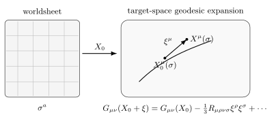
The equal-scale great-circle section uses a unit sphere, $X_0=(0,0,1)$, and $\xi=(\pi/3,0,0)$. Its exponential-map curve is $X_s=(\sin(\pi s/3),0,\cos(\pi s/3))$, $0\le s\le1$. The tangent vector, geodesic arc, and chord are different geometric objects; the fluctuation expansion uses the first to define the second.

Isolating the logarithm without confusing it with an infrared divergence

Use an orthonormal target frame for the fluctuation and write

$$S_2=\frac1{4\pi\alpha'}\int d^2\sigma\, \xi^i\mathscr L_{ij}\xi^j, \qquad \mathscr L=-D_aD_a+\mathsf Q, \qquad \operatorname{tr}\mathsf Q=-R_{\mu\nu}\partial_aX_0^\mu\partial_aX_0^\nu.$$

The Gaussian integral contributes $\Gamma_1=\tfrac12\operatorname{Tr}\log\mathscr L$. The overall kinetic normalization changes a background-independent determinant, not the coefficient of the curvature term.

Continue the worldsheet dimension to $d=2-\epsilon$ and introduce a small auxiliary infrared mass $m_{\rm IR}$. The coincident free inverse operator is

$$I_d(m_{\rm IR}) =\int\frac{d^dp}{(2\pi)^d}\frac1{p^2+m_{\rm IR}^2} =\frac{\Gamma(1-d/2)}{(4\pi)^{d/2}} (m_{\rm IR}^2)^{d/2-1}.$$

This follows by inserting $1/(p^2+m^2)=\int_0^\infty ds\,e^{-s(p^2+m^2)}$ and doing the Gaussian momentum integral. Near two dimensions, $I_d=1/(2\pi\epsilon)+O(1)$. The mass separates the ultraviolet pole from the infrared divergence: setting $m_{\rm IR}=0$ before evaluating the integral would give a scaleless dimensional integral and conceal this separation.

Expanding the determinant to first order in the curvature endomorphism gives

$$\Gamma_{1,\rm div} =\frac12 I_d\int d^2\sigma\,\operatorname{tr}\mathsf Q =-\frac1{4\pi\epsilon}\int d^2\sigma\, R_{\mu\nu}\partial_aX_0^\mu\partial_aX_0^\nu.$$

The pullback connection is needed for covariance. At this order it supplies no additional independent scalar divergence: its curvature is antisymmetric in worldsheet indices, while a curvature-squared invariant has four worldsheet derivatives. In a covariant regulator this is the first local coefficient of the Laplace-type determinant. The calculation concerns the logarithmic kinetic counterterm; it is not a calculation of power-divergent vacuum terms or the curved-worldsheet central anomaly.

The counterterm cancels $\Gamma_{1,\rm div}$, so its sign is positive. Denoting the dimensionally continued bare metric by $G^{\rm bare}$ gives minimal subtraction in the form

$$G^{\rm bare}_{\mu\nu} =\mu^{-\epsilon}\left[G_{\mu\nu}(\mu) +\frac{\alpha'}{\epsilon}R_{\mu\nu}[G(\mu)]+\cdots\right].$$

At fixed bare metric, differentiation with respect to $\log\mu$ yields

$$\mu\frac{dG_{\mu\nu}}{d\mu} =\epsilon G_{\mu\nu}+\alpha'R_{\mu\nu}+O(\alpha'^2), \qquad \beta^G_{\mu\nu}=\alpha'R_{\mu\nu}+O(\alpha'^2) \quad(d=2).$$

At this order the derivative of the Ricci counterterm under the classical uniform rescaling of $G$ is zero, because $R_{\mu\nu}$ with both indices down is unchanged by a constant metric rescaling. This is why no extra term is lost in extracting the finite coefficient. The dimensionally regulated bare-coupling method is discussed in Callan and Thorlacius §4; their $2+\epsilon$ regulator uses the opposite sign for $\epsilon$.

A momentum shell gives the same sign transparently:

$$\int_{\mu<|p|<\Lambda}\frac{d^2p}{(2\pi)^2p^2} =\frac1{2\pi}\log\frac\Lambda\mu, \qquad G(\mu)=G(\Lambda)-\alpha'R\log\frac\Lambda\mu+\cdots.$$

Integrating out short wavelengths therefore decreases a positively curved metric toward the infrared. Defining the flow parameter toward the ultraviolet, as $\log\mu$, instead gives $+\alpha'R$. These are the same running described in opposite directions.

The O(N) model and the meaning of RG flow

The round sphere supplies a concrete normalization check. Let $n^A n^A=1$, $A=1,\ldots,N$, so the target is $S^{N-1}$ with radius $R$. Its action is

$$S=\frac{R^2}{4\pi\alpha'}\int d^2\sigma\,(\partial_an^A)^2 =\frac1{2g}\int d^2\sigma\,(\partial_an^A)^2, \qquad g=\frac{2\pi\alpha'}{R^2}.$$

The $N$ here counts embedding components; the sphere has $N-1$ tangent directions. Writing $G_{ij}=R^2\widehat G_{ij}$ with the unit-sphere metric, its Ricci tensor is $R_{ij}=(N-2)\widehat G_{ij}$. Consequently,

$$\frac{dR^2}{d\log\mu}=\alpha'(N-2)+\cdots, \qquad \beta_g=-\frac{N-2}{2\pi}g^2+O(g^3).$$

For $N>2$, weak coupling improves toward the ultraviolet: the model is asymptotically free. Toward the infrared the sphere shrinks in string units and the perturbative expansion fails. This running does not by itself prove the nonperturbative mass gap or identify its spectrum. Nor does an arbitrary running sigma model define a Weyl-invariant string background.

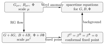
The one-loop example has $t=\log(\mu/\mu_0)$ and $R^2/\alpha'=4+t$ on $-3\le t\le3$. The separate coupling axis shows $g=2\pi/(4+t)$. The shading at $-3\le t\le-2$ is a qualitative warning of small radius, not a sharp validity threshold; the one-loop approximation loses control as curvature grows. The variable $t$ is a worldsheet RG parameter, not a target-space time coordinate.

Weyl coefficients and the spacetime equations

Why the dilaton changes the condition

The kinetic and two-form terms are classically Weyl invariant in two dimensions. A nonconstant dilaton coupling is not. Under $\delta\gamma_{ab}=2\omega\gamma_{ab}$,

$$\delta_\omega S_\Phi =-\frac1{2\pi}\int d^2\sigma\sqrt\gamma\, \Phi\nabla_{\rm ws}^2\omega =-\frac1{2\pi}\int d^2\sigma\sqrt\gamma\, \omega\nabla_{\rm ws}^2\Phi(X),$$

on a closed surface. The subscript distinguishes the worldsheet Laplacian acting on $\Phi(X(\sigma))$ from a target-space Laplacian acting on $\Phi(x)$. Even on a flat worldsheet, where $S_\Phi$ vanishes, its metric variation need not vanish.

Ordinary beta functions describe scale dependence of couplings. Weyl-anomaly coefficients also include this improvement and the freedom to redefine the map $X$. Denote them by $\bar\beta$. To the order considered here, the improvement acts as a target diffeomorphism with vector $v^\mu=\alpha'\nabla^\mu\Phi$:

$$\bar\beta^G=\beta^G+\mathcal L_vG, \qquad \bar\beta^B=\beta^B+\iota_vH.$$

For $B$, the equality is modulo an exact two-form, because $\mathcal L_vB=\iota_vH+d(\iota_vB)$. Thus $\mathcal L_vG=2\alpha'\nabla_\mu\nabla_\nu\Phi$. A flat-worldsheet RG flow can be a redundant coordinate change rather than a physical change of the theory; the local Weyl condition tests whether the improvement cancels it.

The leading massless coefficients

In covariant field variables appropriate to the two-derivative string action, the coefficients are

$$\bar\beta^G_{\mu\nu} =\alpha'\left(R_{\mu\nu}+2\nabla_\mu\nabla_\nu\Phi -\frac14H_{\mu\rho\sigma}H_\nu{}^{\rho\sigma}\right) +O(\alpha'^2),$$ $$\bar\beta^B_{\mu\nu} =\alpha'\left(-\frac12\nabla^\lambda H_{\lambda\mu\nu} +\nabla^\lambda\Phi\,H_{\lambda\mu\nu}\right)+O(\alpha'^2),$$ $$\bar\beta^\Phi =\frac{D-26}{6} +\alpha'\left[(\nabla\Phi)^2-\frac12\nabla^2\Phi -\frac1{24}H^2\right]+O(\alpha'^2).$$

The Ricci coefficient was derived above. The two-form contributions and the general dilaton coefficient are the additional curved-background results discussed by Callan and Thorlacius §§3.3–3.5 and Tong §7.2.3, translated into this choice of coefficients. They are not consequences of the metric loop alone. In particular, the dilaton coefficient includes the central anomaly and improvement terms; counting its diagrams as simply the same one-loop metric calculation would be misleading.

For a background with no other turned-on couplings, local Weyl invariance requires all three $\bar\beta$ to vanish. Higher-order coefficients depend on local field redefinitions and subtraction scheme. The leading equations displayed here are controlled for sufficiently small curvature and field gradients; balancing an order-one central deficit against a large gradient requires additional information. The exact linear CFT below supplies that information in one special case.

The dilaton equation is a trace combination

Define the tensors already derived from the effective action,

$$\begin{aligned} \mathcal E_{\mu\nu}&=R_{\mu\nu}+2\nabla_\mu\nabla_\nu\Phi -\frac14H_{\mu\rho\sigma}H_\nu{}^{\rho\sigma},\\ \mathcal D_\Phi&=R+4\nabla^2\Phi-4(\nabla\Phi)^2-\frac1{12}H^2-C, \qquad C=\frac{2(D-26)}{3\alpha'}. \end{aligned}$$

Taking the target trace of the metric coefficient gives the useful identities

$$\begin{aligned} \bar\beta^\Phi-\frac14G^{\mu\nu}\bar\beta^G_{\mu\nu} &=-\frac{\alpha'}4\mathcal D_\Phi+O(\alpha'^2),\\ \bar\beta^B_{\mu\nu} &=-\frac{\alpha'}2e^{2\Phi}\nabla^\lambda \left(e^{-2\Phi}H_{\lambda\mu\nu}\right)+O(\alpha'^2). \end{aligned}$$

For example, the $H^2$ coefficient in the first line is $-1/24+1/16=1/48$, exactly the coefficient obtained from $-\mathcal D_\Phi/4$. The resulting simultaneous equations are the bulk equations of

$$S_{\rm S}^{(2)}=\frac1{2\kappa_{D,0}^2}\int d^Dx\sqrt{-G}\,e^{-2\Phi} \left[R+4(\nabla\Phi)^2-\frac1{12}H^2-C\right].$$

Its raw inverse-metric Euler tensor is $\mathcal E_{\mu\nu}-G_{\mu\nu}\mathcal D_\Phi/2$, and its dilaton Euler derivative is proportional to $-2\mathcal D_\Phi$. Therefore neither $\bar\beta^\Phi$ alone nor $\bar\beta^G$ alone should be identified with the corresponding raw variational derivative. The simultaneous vanishing conditions agree at the displayed order. The overall gravitational coupling is not determined by setting beta functions to zero.

The exact linear-dilaton CFT

Take a flat target, no two-form, and

$$\Phi(X)=\Phi_0+V_\mu X^\mu, \qquad G_{\mu\nu}=\eta_{\mu\nu},\qquad H=0.$$

Here $V$ is constant with dimension inverse length. The number $\Phi_0$ is the value at the coordinate origin, not an assumed finite asymptotic dilaton. The local flat-worldsheet theory is Gaussian, but its stress tensor remembers the curvature coupling.

Deriving the improvement and all stress-tensor poles

In two dimensions, varying the curvature coupling with respect to the inverse metric gives, up to a boundary term,

$$\delta S_\Phi=\frac1{4\pi}\int\sqrt\gamma\, \left(\gamma_{ab}\nabla_{\rm ws}^2\Phi -\nabla_a\nabla_b\Phi\right)\delta\gamma^{ab}.$$

Using the overview’s relation between the metric stress tensor and $T(z)$, its flat-plane contribution is $+\partial^2\Phi$. Hence

$$T=T_0+A,\qquad T_0=-\frac1{\alpha'}:J\cdot J:, \qquad J^\mu=\partial X^\mu, \qquad A=V\cdot\partial J.$$

The sign follows from the inverse-metric variation, not from the desired central charge. At separated points put $u=z-w$. Differentiating the free-field contraction gives

$$J^\mu(z)J^\nu(w)\sim-\frac{\alpha'\eta^{\mu\nu}}{2u^2}, \qquad \partial J^\mu(z)\partial J^\nu(w) \sim\frac{3\alpha'\eta^{\mu\nu}}{u^4}.$$

The free $T_0T_0$ OPE has central coefficient $D/2$ and the usual second and first poles. The remaining terms are

$$\begin{aligned} T_0(z)A(w)&\sim\frac{2V\cdot J}{u^3} +\frac{2A}{u^2}+\frac{\partial A}{u},\\ A(z)T_0(w)&\sim-\frac{2V\cdot J}{u^3}, & A(z)A(w)&\sim\frac{3\alpha'V^2}{u^4}. \end{aligned}$$

The operators on the right are evaluated at $w$. The third-order poles cancel between the two cross terms. The last expression is one elementary contraction of differentiated fields, not a double Wick pairing. Adding the terms gives the full singular OPE

$$T(z)T(w)\sim\frac{D/2+3\alpha'V^2}{u^4} +\frac{2T(w)}{u^2}+\frac{\partial T(w)}u, \qquad c_m=D+6\alpha'V^2.$$

The ghost central charge is $-26$. Thus local criticality requires

$$c_m=26,\qquad V^2=\frac{26-D}{6\alpha'}.$$

This agrees with $\bar\beta^\Phi=0$, while the metric and two-form coefficients vanish. More strongly, the Gaussian OPE calculation is exact: there are no additional interacting matter vertices to renormalize these local CFT data. It does not establish weak coupling at every target point or supply boundary conditions in a strongly coupled region.

With a real Lorentzian target and $D\ge2$, the required gradient can be spacelike for $D<26$, timelike for $D>26$, or null for $D=26$. In the last case both $V=0$ and nonzero null $V$ are possible. A chosen nonzero vector breaks part of target-space Poincaré symmetry; it does not evade the critical-dimension result for a Poincaré-invariant flat vacuum with constant dilaton.

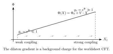
For the spacelike example $u=V\cdot X$ and $\Phi_0=-2$, the plotted local coupling is $e^{\Phi}=e^{u-2}$ on $-2\le u\le4$; it equals one at $u=2$. These are dimensionless axes with linear plotting scales. The shaded region $u\ge2$ is not weakly coupled. Continuing toward large positive $u$ requires strong-coupling information even though the local worldsheet CFT is Gaussian.

Exponential weights and the background charge

For $\mathcal V_k=:e^{ik\cdot X}:$, the improvement has the contraction

$$V\cdot\partial^2X(z)\,\mathcal V_k(w) \sim\frac{i\alpha'V\cdot k}{2u^2}\mathcal V_k(w).$$

Together with the free-stress contraction, this gives

$$T(z)\mathcal V_k(w)\sim\frac{h(k)\mathcal V_k(w)}{u^2} +\frac{\partial\mathcal V_k(w)}u, \qquad h(k)=\bar h(k)=\frac{\alpha'}4\left(k^2+2iV\cdot k\right).$$

Unlike the central charge, the linear term in this weight tests the sign of the improvement. Real $k$ can give a complex weight; the plane waves appropriate to the weighted target measure instead involve a shifted momentum. For real $p$ and $V$,

$$k=p-iV, \qquad e^{ik\cdot x}=e^{V\cdot x}e^{ip\cdot x}, \qquad h=\frac{\alpha'}4(p^2+V^2).$$

This is also visible in the zero mode. On a closed genus-$g$ surface, its formal dependence is

$$\int d^Dx_0\, \exp\left[i\Bigl(\sum_i k_i\Bigr)\cdot x_0-\chi V\cdot x_0\right], \qquad \chi=2-2g.$$

The background-charge condition is therefore $\sum_i k_i+i\chi V=0$. For a real spacelike $V$, the ordinary real zero-mode integral need not converge. This equation is a neutrality condition in an analytically continued or otherwise specified prescription, not automatically a usual real-momentum delta function. Exercise 5 relates its sphere pairing to the weighted target-space norm. Tong §7.4.4 discusses the linear CFT; the improvement and signs here follow directly from the stated action variation.

The shifted tachyon spectrum and its limits

Let $\mathcal T(x)$ denote the spacetime tachyon fluctuation, to distinguish it from the worldsheet stress tensor. Absorb its constant normalization into the field and use the quadratic string-frame action

$$S_{\mathcal T}=-\frac12\int d^Dx\,e^{-2\Phi} \left[(\partial\mathcal T)^2+m_T^2\mathcal T^2\right], \qquad m_T^2=-\frac4{\alpha'}.$$

Its equation is $(\Box-2V\cdot\partial-m_T^2)\mathcal T=0$. Now set $\mathcal T=e^\Phi\widehat{\mathcal T}$. For a constant gradient,

$$e^{-2\Phi}(\partial\mathcal T)^2 =(\partial\widehat{\mathcal T})^2 +V\cdot\partial(\widehat{\mathcal T}^{2}) +V^2\widehat{\mathcal T}^{2}.$$

With vanishing boundary contributions, the middle term integrates to zero. The canonically weighted field therefore has

$$S_{\mathcal T}=-\frac12\int d^Dx \left[(\partial\widehat{\mathcal T})^2+m_{\rm eff}^2\widehat{\mathcal T}^{2}\right], \qquad m_{\rm eff}^2=m_T^2+V^2=\frac{2-D}{6\alpha'}.$$

The CFT gives the same result without a derivative-expansion assumption: $h=\bar h=1$ implies $p^2+V^2=4/\alpha'$, or $p^2=-m_{\rm eff}^2$. This exact linearized mass-shell statement is why the simple quadratic action remains useful even when $\alpha'V^2$ is not small.

For $D=2$, this mode is massless. That does not prove stability of a complete interacting two-dimensional string background. The field redefinition changes the form of interactions, the strong-coupling end remains, and a physical spectrum requires a choice of allowed wave functions and target-space boundary conditions. For a timelike gradient the background is time dependent, so a constant coefficient in this transformed wave equation is not by itself a stationary-particle interpretation. No nonsingular nonlinear endpoint of tachyon evolution follows from this calculation; Tong §7.4.5 discusses why the tachyon remains an essential limitation of the bosonic backgrounds.

Exercises

1. An explicit second variation on a sphere

On a unit $S^2\subset\mathbb R^3$, take $X_0(x,y)=(\cos qx,\sin qx,0)$ with periodic $x$. Let $e_t=(-\sin qx,\cos qx,0)$ and $e_n=(0,0,1)$. For $\xi=h(x,y)e_t+f(x,y)e_n$, derive the quadratic kinetic density by differentiating the exact exponential map. What do the normal Fourier modes say about the sign of the Hessian? Explain why this does not reverse the ultraviolet counterterm.

Solution

Both frame vectors are covariantly parallel along the great circle: the ordinary derivative of $e_t$ is normal to the sphere and projects out of $D_xe_t$. Set $r^2=h^2+f^2$. The exact map and its expansion are

$$X_s=\cos(sr)X_0+\frac{\sin(sr)}r\xi =X_0+s\xi-\frac{s^2r^2}{2}X_0+O(s^3).$$

The expression is smooth at $r=0$ by its limiting value. Differentiation gives

$$\partial_x\xi=h_xe_t-qhX_0+f_xe_n, \qquad \partial_y\xi=h_ye_t+f_ye_n.$$

The $s^2$ coefficient in $\sum_a|\partial_aX_s|^2$ is $\sum_a|\partial_a\xi|^2-q^2r^2$. Thus

$$\mathcal L_2=(\partial h)^2+(\partial f)^2-q^2f^2.$$

The tangent $h^2$ terms cancel. Geometrically, only fluctuations perpendicular to the geodesic feel this sectional-curvature potential. This directly checks the full Hessian rather than only the normal-coordinate metric expansion.

On a rectangular worldsheet torus with side lengths $L_x,L_y$, choose $qL_x=2\pi w$ with integer $w$. The normal eigenvalues are

$$\lambda_{n,m}=\left(\frac{2\pi n}{L_x}\right)^2 +\left(\frac{2\pi m}{L_y}\right)^2-q^2.$$

Some low modes are negative for $q\ne0$: the winding great-circle map is a stationary point, not a local minimum among maps into $S^2$. A negative low mode affects the infrared saddle interpretation, while the ultraviolet logarithm comes from momenta much larger than $|q|$. One may isolate that ultraviolet coefficient with an infrared regulator or a suitable analytic continuation of the saddle. Replacing the curvature term by $+q^2f^2$ would change the actual second variation and would give the wrong counterterm sign.

2. Running radius and dimensional transmutation

Integrate the one-loop O(N) beta function from a scale $\mu_0$ with coupling $g_0$. Express the result in terms of an RG-invariant scale for $N>2$. Determine the scale at which $R^2=\alpha'$ in the plotted O(3) example, and explain the cases $N=2$ and $N=1$.

Solution

Since $d(1/g)/d\log\mu=(N-2)/(2\pi)$,

$$\frac1{g(\mu)}=\frac1{g_0}+\frac{N-2}{2\pi}\log\frac\mu{\mu_0}, \qquad \Lambda_\sigma=\mu_0\exp\left[-\frac{2\pi}{(N-2)g_0}\right].$$

Equivalently, $g(\mu)=2\pi/[(N-2)\log(\mu/\Lambda_\sigma)]$ in the weak-coupling region. Differentiating $\Lambda_\sigma$ using the one-loop beta function gives zero at this order. This is dimensional transmutation: a dimensionless reference coupling is replaced by a scale. Higher orders change this simple formula and its scheme dependence.

The radius obeys

$$\frac{R^2(\mu)}{\alpha'}=\frac{R_0^2}{\alpha'}+(N-2)\log\frac\mu{\mu_0}.$$

For $N=3$ and $R_0^2/\alpha'=4$, the radius reaches one string unit at $\mu=\mu_0e^{-3}$. The formal zero occurs later at $\mu=\mu_0e^{-4}=\Lambda_\sigma$, where the weak-curvature approximation has already failed. Neither the zero radius nor a continued negative $R^2$ is a trustworthy prediction of the one-loop formula.

For $N=2$ the target is a circle, whose intrinsic Ricci tensor vanishes. The smooth sigma model is a compact free boson and has no perturbative radius running; possible vortex perturbations require additional operators and data. For $N=1$, $S^0$ is two points, not a smooth positive-dimensional sigma-model target. Substituting $N=1$ into a formula derived with tangent fluctuations does not describe an ordinary interacting sphere sigma model.

3. Metric and two-form equations do not fix the central deficit

Consider a round $S^3$ of radius $R$ times flat spectator directions. In an orthonormal sphere frame, take $H_{abc}=q_H\epsilon_{abc}$, with constant $q_H$ and constant dilaton. Solve the leading metric and two-form Weyl conditions. Does this also solve the dilaton condition in $D=26$? If not, add a linear dilaton along a flat spacelike spectator and determine its required norm. State the approximation being used.

Solution

On the sphere, $R_{ab}=2\delta_{ab}/R^2$, while

$$H_{acd}H_b{}^{cd}=2q_H^2\delta_{ab}, \qquad H^2=6q_H^2.$$

The volume form is covariantly constant, so $\nabla^aH_{abc}=0$. The metric equation requires $2/R^2-q_H^2/2=0$, hence $q_H^2=4/R^2$. Both tensor Weyl coefficients then vanish, but

$$\bar\beta^\Phi=\frac{D-26}{6}-\frac{\alpha'q_H^2}{4} =\frac{D-26}{6}-\frac{\alpha'}{R^2}$$

at the displayed order. At $D=26$ this is nonzero. Equivalently, the scalar action equation gives $\mathcal D_\Phi=6/R^2-2/R^2=4/R^2$, in agreement with $\bar\beta^\Phi=-\alpha'\mathcal D_\Phi/4$ once the metric trace vanishes.

A constant gradient $V$ along a flat spectator has zero Hessian and no contraction with $H$. It leaves the tensor equations unchanged but adds $\alpha'V^2$ to $\bar\beta^\Phi$. Thus $V^2=1/R^2$ cancels the leading deficit in $D=26$.

This is a local leading-order background calculation, controlled for $\alpha'/R^2\ll1$. A global string construction must also impose flux quantization and specify the exact curved-factor CFT and its higher-order radius relation. The exercise does not derive those extra conditions or claim this classical radius relation is exact. It illustrates why solving only the metric and two-form equations leaves a scalar central-charge condition.

4. Improved Virasoro modes and a sign-sensitive Ward identity

Using the oscillator expansion of $\partial X$, derive the Virasoro modes in the linear-dilaton theory. Verify their full commutator, including the change of central charge. Then calculate $T(z)\partial X^\mu(w)$ and explain why the result contains a sign test absent from the central charge alone.

Solution

The holomorphic expansion is $\partial X^\mu=-i\sqrt{\alpha'/2}\sum_n\alpha_n^\mu z^{-n-1}$. Differentiating once gives

$$L_n=L_n^{(0)}+I_n, \qquad I_n=i\sqrt{\frac{\alpha'}2}(n+1)V\cdot\alpha_n.$$

Use $[L_m^{(0)},\alpha_n^\mu]=-n\alpha_{m+n}^\mu$. The cross commutators are

$$[L_m^{(0)},I_n]+[I_m,L_n^{(0)}] =i\sqrt{\frac{\alpha'}2}\bigl[m(m+1)-n(n+1)\bigr]V\cdot\alpha_{m+n} =(m-n)I_{m+n}.$$

The improvement commutator is central. Setting $n=-m$ after using the oscillator delta function gives

$$[I_m,I_n]=\frac{\alpha'V^2}{2}(m^3-m)\delta_{m+n,0}.$$

Adding the free algebra therefore yields

$$[L_m,L_n]=(m-n)L_{m+n} +\frac{D+6\alpha'V^2}{12}(m^3-m)\delta_{m+n,0}.$$

This includes the $-m$ term, so the global modes have no central extension. It is the algebra of the improved stress tensor; a physical adjoint and state pairing must include the background charge rather than being inferred from the flat zero-mode vacuum.

The current OPE follows from one extra differentiated contraction:

$$T(z)J^\mu(w)\sim\frac{\alpha'V^\mu}{(z-w)^3} +\frac{J^\mu(w)}{(z-w)^2}+\frac{\partial J^\mu(w)}{z-w}.$$

Thus the positive contour action gives

$$\delta_\epsilon J^\mu =\epsilon\partial J^\mu+(\partial\epsilon)J^\mu +\frac{\alpha'}2V^\mu\partial^2\epsilon.$$

Changing $V$ to $-V$ leaves $c$ unchanged but reverses this extra term and the linear term in $h(k)$. The current is not an ordinary weight-one primary in the improved theory. The positive contour sign is the active transformation used on the conformal-transformation page.

5. Background charge, two-point pairing, and weighted momentum

Derive the formal genus-$g$ neutrality condition from the constant mode of $X$. On the sphere find the momentum paired with $k$, verify equality of their conformal weights, and relate the answer to modes with $k=p-iV$. Explain when the corresponding target-space pairing is positive and what remains to be specified for a noncompact linear dilaton.

Solution

Gauss–Bonnet gives $\int\sqrt\gamma R^{(2)}=4\pi\chi$. A constant shift $X\mapsto X+x_0$ therefore changes the dilaton action by $\chi V\cdot x_0$. Combined with the vertex exponentials, the zero-mode dependence is $\exp[(i\sum k_i-\chi V)\cdot x_0]$. The formal neutrality requirement is

$$\sum_i k_i=-i\chi V.$$

On a sphere, $\chi=2$, and a two-point pairing has $k'=-k-2iV$. Substitution gives

$$k'^2+2iV\cdot k'=k^2+2iV\cdot k,$$

so the paired operators have equal weights. For $k=p-iV$ with real $p,V$, the partner is $k'=-p-iV=-k^*$. In target space the corresponding modes are proportional to $e^\Phi e^{ip\cdot x}$, with the constant $e^{\Phi_0}$ absorbed into their normalization. Their weighted product is

$$e^{-2\Phi}\left(e^\Phi e^{ip'\cdot x}\right)^* \left(e^\Phi e^{ip\cdot x}\right) =e^{i(p-p')\cdot x}.$$

For a real spacelike profile on a spatial slice, the weight $e^{-2\Phi}$ is positive. With suitable boundary conditions it defines the usual positive scalar spatial pairing; plane waves are delta-normalized generalized modes, not square-integrable states. This is not a claim of positive norm for the entire Lorentzian worldsheet Fock space.

At genus one, $\chi=0$, so the formal selection is unshifted. At higher genus the shift changes with $\chi$. Along a noncompact real gradient the unregulated worldsheet zero-mode integral can diverge at an end; an analytic continuation, wave packets, a wall, or a completed background must specify how correlators are defined. Formal neutrality does not supply that prescription by itself.

6. Conjugating the tachyon operator for a general profile

Keep a flat target but allow an arbitrary smooth $\Phi(x)$. Starting with the quadratic weighted tachyon action, derive the differential operator and its conjugate under $\mathcal T=e^\Phi\widehat{\mathcal T}$. Identify the position-dependent mass coefficient, specialize to a critical linear dilaton, and determine how a local cubic interaction transforms. Compare $D=2$ and $D=26$.

Solution

Varying the action, with the same weight retained in the integration by parts, gives

$$\mathscr D\mathcal T=0, \qquad \mathscr D=\Box-2\partial_\mu\Phi\,\partial^\mu-m_T^2.$$

Direct differentiation, without dropping a boundary term, yields the operator identity

$$e^{-\Phi}\mathscr D e^\Phi =\Box-m_T^2-(\partial\Phi)^2+\Box\Phi.$$

The action gives the same result: the cross term is $\partial_\mu\Phi\,\partial^\mu(\widehat{\mathcal T}^{2})$, whose integral is $-\Box\Phi\,\widehat{\mathcal T}^{2}$ when the surface term vanishes. Hence

$$m_{\rm eff}^2(x)=m_T^2+(\partial\Phi)^2-\Box\Phi.$$

This general profile need not satisfy the string background equations; the identity is a field transformation of the supplied quadratic action. For a linear profile, $\Box\Phi=0$ and criticality fixes $V^2=(26-D)/(6\alpha')$, giving $m_{\rm eff}^2=(2-D)/(6\alpha')$. At $D=2$ the coefficient vanishes. At $D=26$ it is the usual $-4/\alpha'$, including for a nonzero null gradient. The $D=2$ statement is made directly in string-frame variables and does not use an Einstein-frame rescaling singular at $D=2$.

Finally, a term $\int e^{-2\Phi}\lambda_3\mathcal T^3$ becomes $\int\lambda_3e^\Phi\widehat{\mathcal T}^{3}$. Even when the quadratic coefficient is nonnegative, interactions become strong where $e^\Phi$ grows. The spectrum of the linear equation, normalizability at the ends, and stability of a nonlinear completion are distinct questions.

References

• Callan, Curtis G., Jr., and Lárus Thorlacius. “Sigma Models and String Theory.” In Particles, Strings and Supernovae, proceedings of TASI 1988, vol. 2, edited by Antal Jevicki and Chung-I Tan, World Scientific (1989), pp. 795–878. §§3.2–3.5 and 4. Lecture text.
• Tong, David. Lectures on String Theory. University of Cambridge Part III lecture notes (2009; arXiv version 3, 2012), §§7.1.1, 7.2.3, and 7.4.4–7.4.5. arXiv:0908.0333.