M-Theory Origin of Type IIA Branes

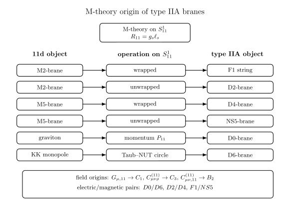
Type IIA string theory relates the dilaton to the size of an eleventh dimension. Its D0 charge becomes circle momentum; its strings and higher branes arise from membranes, fivebranes, and circle geometry. This explains their tensions and connects several apparently different supergravity solutions. Making the connection quantitative requires both the normalization of the fields and the distinction between a localized source and a source spread around a circle.

We use the shared eleven-dimensional fields and circle normalization, together with the RR potentials and brane couplings. The discussion concerns massless IIA, classical two-derivative exterior solutions, and sources with vanishing worldvolume flux. The preceding page supplies the ten-dimensional backgrounds and their charge normalization.

The D0 tower and the circle radius

A D0-brane has mass $T_0=1/(g_s\ell_s)$. If a normalizable BPS state with D0 charge $n_0$ exists, its mass is

$$M_{n_0}=\frac{|n_0|}{g_s\ell_s}.$$

Compare this with a massless eleven-dimensional particle carrying circle momentum $p_z=n/R_{11}$: in the ten-dimensional rest frame, the mass shell condition gives $M=|n|/R_{11}$. The two spectra identify $R_{11}=g_s\ell_s$. Reduction of the Einstein term then gives

$$2\kappa_{11}^2=(2\pi R_{11})\,2\kappa_{10}^2, \qquad \ell_p^9=R_{11}g_s^2\ell_s^8,$$

and hence $\ell_p^3=g_s\ell_s^3$. These comparisons use metrics that agree in the noncompact directions at infinity. Comparing a mass measured in one metric with a radius measured in a differently rescaled metric would miss the powers of $g_s$.

The existence of a state is an additional question. Several widely separated D0-branes have a continuum beginning at the same BPS threshold. The mass formula does not decide whether their relative quantum mechanics also has a normalizable state at threshold, or whether it is unique. Witten, section 2, develops the circle interpretation; Sethi and Stern establish existence for two D0-branes by a separate index analysis. A protected mass and a bound-state existence argument play different roles.

Which sign of circle momentum carries positive D0 charge?

The connection in the metric is $\eta=dz-g_sC_1$. Its horizontal vector is $\partial_\mu+g_sC_\mu\partial_z$. Acting on a Fourier mode gives

$$\left(\partial_\mu+g_sC_\mu\partial_z\right) \left[e^{inz/R_{11}}\psi(x)\right] =e^{inz/R_{11}}\left(\partial_\mu+i\frac{g_sn}{R_{11}}C_\mu\right)\psi.$$

Relative to a worldline coupling $+q\int C_1$, the covariant derivative is $\partial-iqC_1$. Thus

$$q=-g_sp_z=-\frac{g_sn}{R_{11}}, \qquad n=-n_0.$$

The sign follows from the connection and source coupling; the absolute mass cannot fix it. For example, the positive D0 solution has $g_sC_1=(H^{-1}-1)dt$. Its lift is

$$ds_{11}^2=-dt^2+dz^2+(H-1)(dt+dz)^2+dx_\perp^2.$$

It is a gravitational wave traveling toward decreasing $z$, consistent with negative $p_z$ for positive D0 charge. Exercise 1 obtains the same sign directly from the particle action.

Reducing the fields and the source actions

The bosonic eleven-dimensional action and its exterior field equations are

$$S_{11}=\frac1{2\kappa_{11}^2} \left[\int\left(R*1-\frac12\mathcal F_4\wedge *\mathcal F_4\right) -\frac16\int\mathcal A_3\wedge\mathcal F_4\wedge\mathcal F_4\right],$$ $$\begin{aligned} d\mathcal F_4&=0, &d*\mathcal F_4+\tfrac12\mathcal F_4\wedge\mathcal F_4&=0,\\ R_{MN}&=\frac1{12}\left(\mathcal F_{MPQR}\mathcal F_N{}^{PQR} -\frac1{12}G_{MN}\mathcal F_{PQRS}\mathcal F^{PQRS}\right). \end{aligned}$$

The factor in the Einstein equation includes trace reversal in eleven dimensions. The first two equations hold away from magnetic and electric sources. The action and reduction are discussed in Saffin, appendix A; the earlier action calculation derives their translation to the fields used here.

Differentiate the shared three-form ansatz and regroup it into horizontal and circle components:

$$\begin{aligned} \mathcal F_4 &=g_s\,dC_3+H_3\wedge dz\\ &=g_s\widetilde F_4+H_3\wedge\eta, &\widetilde F_4&=dC_3-C_1\wedge H_3. \end{aligned}$$

The relative sign uses $H_3\wedge C_1=-C_1\wedge H_3$. It also implies $d\widetilde F_4=-F_2\wedge H_3$. Circle translations with an $x$-dependent parameter require a compensating transformation of $C_3$, as Exercise 1 shows.

The determinant and inverse-metric factors give a useful normalization check:

$$\begin{aligned} \sqrt{-G_{11}}&=e^{-8\phi/3}\sqrt{-G_S},\\ \sqrt{-G_{11}}|\mathcal F_4|_{11}^2 &=\sqrt{-G_S}\left[g_s^2|\widetilde F_4|_S^2 +e^{-2\phi}|H_3|_S^2\right]. \end{aligned}$$

Here $|F_n|^2=F_{M_1\ldots M_n}F^{M_1\ldots M_n}/n!$. The physical coupling $\kappa_{10}$ turns the RR factor into $1/\kappa_{10,0}^2$, while the NS term becomes $e^{-2\Phi}/\kappa_{10,0}^2$. The metric-vector kinetic term similarly carries $g_s^2F_2^2$. Removing the factors of $g_s$ in the lift would therefore change the ten-dimensional action.

Wrapped membranes and fivebranes

For a static M2 lying in three noncompact directions, the induced volume is multiplied by $e^{-\phi}$. Its action becomes the D2 DBI action because

$$T_{\rm M2}e^{-\phi}=T_2e^{-\phi}=\mu_2e^{-\Phi}, \qquad g_sT_{\rm M2}=\mu_2.$$

The second equality fixes the RR source coupling, not just the tension. If a spatial M2 direction wraps the circle, the two noncompact factors $e^{-2\phi/3}$ and the circle factor $e^{4\phi/3}$ cancel in the volume determinant. Circle integration instead gives

$$2\pi R_{11}T_{\rm M2}=\frac1{2\pi\alpha'}=T_{\rm F1}, \qquad T_{\rm M2}\int B_2\wedge dz=T_{\rm F1}\int B_2.$$

An unwrapped M5 has volume factor $e^{-2\phi}$, producing the NS5 dilaton dependence and tension. A wrapped M5 has factor $e^{-\phi}$ and the D4 tension. The asymptotic magnitudes are

Eleven-dimensional object	Circle operation	Ten-dimensional object and tension
M2	unwrapped	D2: $T_2=T_{\rm M2}$
M2	wrapped	F1: $T_{\rm F1}=2\pi R_{11}T_{\rm M2}$
M5	unwrapped	NS5: $T_{\rm NS5}=T_{\rm M5}$
M5	wrapped	D4: $T_4=2\pi R_{11}T_{\rm M5}$
massless particle	circle momentum	D0: $M=\lvert n\rvert/R_{11}$
circle monopole	nontrivial circle bundle	D6

The “unwrapped” entries specify the source dictionary. Whether the transverse circle is resolved or averaged is a separate geometric question.

The orientation of a wrapped M5

Charge needs one more check. Set $B_2=C_1=0$ in a pure single-charge sector. For a horizontal four-form the warped Hodge star gives

$$*_{11}(g_s\mathcal F_4^{\rm IIA}) =g_s(*_S\mathcal F_4^{\rm IIA})\wedge dz =-g_s\mathcal F_6^{\rm IIA}\wedge dz.$$

The last equality uses the shared democratic relation, $\mathcal F_6^{\rm IIA}=-*_S\mathcal F_4^{\rm IIA}$. In this sector the CS product vanishes, so locally

$$\mathcal A_6=-g_sC_5^{\rm WZ}\wedge dz.$$

A positive D4 with worldvolume orientation $dt\wedge dx^1\wedge\cdots\wedge dx^4$ is therefore produced by a wrapped M5 with orientation $-dt\wedge dx^1\wedge\cdots\wedge dx^4\wedge dz$. The two minus signs give $+\mu_4\int C_5^{\rm WZ}$. An unwrapped M5 with orientation $+dt\wedge\cdots\wedge dx^5$ gives the positive NS5. This calculation keeps the dual-potential definition, the circle-last order, and the source orientation together. It does not replace the full M5 worldvolume action in backgrounds with flux.

M2 and M5 geometries and their charge normalization

Let $\omega_d=dt\wedge dx^1\wedge\cdots\wedge dx^{d-1}$ be the stated oriented noncompact worldvolume form. An unwrapped electric M2 and magnetic M5 have metrics

$$\begin{aligned} \text{M2:}\quad ds_{11}^2&=H^{-2/3}ds^2(\mathbb R^{1,2})+H^{1/3}dy_8^2, &\mathcal F_4&=d(H^{-1})\wedge\omega_3,\\ \text{M5:}\quad ds_{11}^2&=H^{-1/3}ds^2(\mathbb R^{1,5})+H^{2/3}dy_5^2, &\mathcal F_4&=-*_{5,\rm flat}dH. \end{aligned}$$

For the M5 line, the coordinate normal orientation completes $\omega_6$ to $\mathrm{vol}_{11}$. Both fields solve the exterior equations when $H$ is a positive harmonic function of the indicated normal coordinates. The equations permit separated aligned centers as well as a single center.

Why a harmonic function solves the coupled equations

Harmonicity is not the whole verification: the form stress tensor must cancel the nonlinear metric terms. Write $v_i=\partial_iH$, $v^2=\delta^{ij}v_iv_j$, and $\Delta H=\delta^{ij}\partial_i\partial_jH$. Direct calculation of the Christoffel symbols gives

$$\begin{array}{c|c|c} & R_{\mu\nu} & R_{ij}\\ \hline \mathrm{M2} &\dfrac{\eta_{\mu\nu}}3\left(\dfrac{\Delta H}{H^2}-\dfrac{v^2}{H^3}\right) &-\dfrac{v_iv_j}{2H^2}+\dfrac{\delta_{ij}v^2}{6H^2}-\dfrac{\delta_{ij}\Delta H}{6H}\\[4pt] \mathrm{M5} &\dfrac{\eta_{\mu\nu}}6\left(\dfrac{\Delta H}{H^2}-\dfrac{v^2}{H^3}\right) &-\dfrac{v_iv_j}{2H^2}+\dfrac{\delta_{ij}v^2}{3H^2}-\dfrac{\delta_{ij}\Delta H}{3H} \end{array}$$

Mixed components vanish. In each row the form stress supplies precisely the terms quadratic in $v_i$. Thus every Einstein component is satisfied when $\Delta H=0$. For the M2 the Maxwell equation reduces to this same condition; the Bianchi identity is automatic. For the M5, $d\mathcal F_4=-(\Delta H)\,d^5y$ gives harmonicity, while $d*\mathcal F_4=0$ follows from the electric dual expression. The CS term vanishes in these purely electric or purely magnetic configurations. Reversing $\mathcal F_4$ preserves the source-free equations, but reverses the charge: flux and source orientation must select the desired brane.

For a single localized center,

$$H_2=1+\frac{Q_2}{r^6}, \qquad H_5=1+\frac{Q_5}{r^3}.$$

The warped electric M2 star simplifies to $*_{11}\mathcal F_4=-*_{8,\rm flat}dH_2$. Its outward flux is therefore $6\Omega_7Q_2$. The outward magnetic M5 flux is $3\Omega_4Q_5$. Equating these to the oriented source strengths yields

$$Q_2=\frac{2\kappa_{11}^2T_{\rm M2}N}{6\Omega_7} =32\pi^2N\ell_p^6, \qquad Q_5=\frac{2\kappa_{11}^2T_{\rm M5}N}{3\Omega_4} =\pi N\ell_p^3.$$

Here $\Omega_7=\pi^4/3$ and $\Omega_4=8\pi^2/3$. These coefficients reproduce the ten-dimensional charges, rather than merely the harmonic powers. For example, wrapping the M2 leaves eight normal directions and gives $Q_{\rm F1}=32\pi^2g_s^2N\alpha'^3$; wrapping the M5 leaves five and gives $Q_{\rm D4}=\pi g_sN\alpha'^{3/2}$, with the oriented source identification derived above.

Near-horizon radii

Define $R_2=Q_2^{1/6}$ and $R_5=Q_5^{1/3}$. In the M2 region $r\ll R_2$, set $u=R_2^3/(2r^2)$. The metric becomes

$$ds_{11}^2=\frac{R_2^2}{4u^2}\left(du^2+ds^2(\mathbb R^{1,2})\right) +R_2^2d\Omega_7^2.$$

Thus the AdS radius is $R_2/2$, whereas the sphere radius is $R_2$. For the M5 region $r\ll R_5$, use $u=2R_5^{3/2}/\sqrt r$:

$$ds_{11}^2=\frac{4R_5^2}{u^2}\left(du^2+ds^2(\mathbb R^{1,5})\right) +R_5^2d\Omega_4^2.$$

The AdS radius is now $2R_5$. If a worldvolume direction was wrapped, this is a local AdS geometry with its inherited periodic identification, not globally uncompactified AdS. For a localized source on a transverse circle, reaching a local uncompactified throat requires both a single-image limit and the near-horizon limit described next.

Localized sources and circle averages

Suppose the M2 circle is transverse, with noncompact normal distance $\rho$ and circle coordinate $z$. A localized periodic array has

$$H_2(\rho,z)=1+Q_2\sum_{m\in\mathbb Z} \frac1{[\rho^2+(z-2\pi mR_{11})^2]^3}.$$

This solution depends on $z$. In contrast, lifting the ten-dimensional D2 background produces a circle-independent harmonic function. The connection between them is the exact zero Fourier mode:

$$\begin{aligned} \overline H_2-1 &=\frac{Q_2}{2\pi R_{11}}\int_{-\infty}^{\infty} \frac{ds}{(\rho^2+s^2)^3}\\ &=\frac{3Q_2}{16R_{11}\rho^5} =\frac{6\pi^2Ng_s\ell_s^5}{\rho^5}. \end{aligned}$$

The integral unfolds one circle cell against all its images; it does not count the images as additional physical charge in that cell. For an M5 on a transverse circle the corresponding calculation is

$$\begin{aligned} H_5(\rho,z)&=1+Q_5\sum_{m\in\mathbb Z} [\rho^2+(z-2\pi mR_{11})^2]^{-3/2},\\ \overline H_5-1&=\frac{Q_5}{2\pi R_{11}}\int_{-\infty}^{\infty} \frac{ds}{(\rho^2+s^2)^{3/2}} =\frac{N\alpha'}{\rho^2}. \end{aligned}$$

The averaged harmonic functions construct the separate smeared M2/D2 and M5/NS5 solutions. Averaging their nonlinear metric components would give different expressions. Moreover, a localized solution without a circle isometry cannot be exactly reduced to just the massless ten-dimensional fields by this averaging operation.

Poisson summation makes the regime of approximation explicit. For $\nu>1/2$ and nonzero real $k$,

$$\int_{-\infty}^{\infty}\frac{e^{-iks}\,ds}{(\rho^2+s^2)^\nu} =\frac{2\sqrt\pi}{\Gamma(\nu)} \left(\frac{|k|}{2\rho}\right)^{\nu-1/2} K_{\nu-1/2}(|k|\rho).$$

The circle harmonics have $k=n/R_{11}$. Since $K_a(x)\sim\sqrt{\pi/(2x)}e^{-x}$ at large $x$, nonzero harmonics are exponentially small for $\rho\gg R_{11}$, with specified power-law prefactors. Close to one image, $s_{\rm loc}=\sqrt{\rho^2+z^2}\ll R_{11}$, that image dominates. A local M2 or M5 throat additionally requires $s_{\rm loc}\ll R_2$ or $R_5$. Neither condition implies the other. Itzhaki and collaborators, sections 3 and 8, use precisely this distinction between circle-independent and localized backgrounds.

At the source’s circle position $z=0$, both panels plot $(H-1)/(\overline H-1)$ against $x=\rho/R_{11}$ on a logarithmic horizontal axis. The additive asymptotic constant is subtracted in both numerator and denominator. The horizontal reference is the circle average. At $x=0.5$, the ratios are about $10.6667$ and $6.29074$; at $x=12$, they are $1.000750$ and $1.000055$. These are harmonic-function comparisons, not averages of the nonlinear metric, and do not by themselves establish a near-horizon limit.

D6 charge as the topology of the circle

The D6 lift is a direct product of its flat seven-dimensional worldvolume and a four-dimensional Taub–NUT metric:

$$ds_{11}^2=ds^2(\mathbb R^{1,6}) +H\left(dr^2+r^2d\Omega_2^2\right)+H^{-1}(dz+A)^2, \qquad A=-g_sC_1.$$

The positive D6 normalization from the preceding page is

$$H=1+\frac{k}{r}, \qquad k=\frac{NR_{11}}2, \qquad \int_{S^2}F_2=-2\pi N\ell_s.$$

It follows that $dA=-*_{3,\rm flat}dH$, whose outward integral is $4\pi k=2\pi NR_{11}$. The negative RR flux and positive circle-bundle charge are compatible because $A=-g_sC_1$.

Choose potentials regular at the north and south poles:

$$A_N=k(1-\cos\theta)d\varphi, \qquad A_S=-k(1+\cos\theta)d\varphi.$$

Their difference is $NR_{11}d\varphi$. The coordinate transition $z_S=z_N+NR_{11}\varphi$ makes $dz_N+A_N=dz_S+A_S$. Dividing by the circle radius gives a dimensionless connection, with first Chern number

$$c_1=\frac1{2\pi}\int_{S^2}\frac{dA}{R_{11}}=N.$$

The factor of $R_{11}$ is essential. The integral of the dimensionful field $F_2=dC_1$ is not itself a dimensionless integer.

The nut and its period

Near $r=0$, put $\rho_4=2\sqrt{kr}$. In a local gauge with $A=-k\cos\theta\,d\varphi$, let $\psi=z/k$. The normal metric approaches

$$ds_4^2=d\rho_4^2+\frac{\rho_4^2}{4} \left[d\theta^2+\sin^2\theta\,d\varphi^2 +(d\psi-\cos\theta\,d\varphi)^2\right], \qquad \Delta\psi=\frac{4\pi}{N}.$$

For $N=1$ this is the smooth polar form of $\mathbb R^4$. For coincident $N>1$, the reduced Hopf period produces $\mathbb R^4/\mathbb Z_N$ at the nut. A multicenter solution with separated unit-charge nuts can instead be smooth at each center. The ten-dimensional circle reduction becomes singular where its fiber shrinks, even when the eleven-dimensional single-nut metric is regular. Itzhaki and collaborators, section 9, exhibit the associated orbifold identifications.

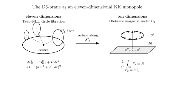
The linking sphere lies in the three-dimensional normal base; the D6 tangent directions are suppressed. Its outward orientation gives positive $\int dA$ and negative $\int F_2$. The circle coordinate transition winds $N$ times. The lower comparison concerns the local Hopf period: one unit gives a smooth nut, whereas coincident $N$ units give an orbifold. The linking sphere is schematic. The lower bars quantitatively compare the coordinate periods for $N=1$ and $N=3$, with length ratio $1:1/3$; their endpoints are identified.

The local radius and the validity of a description

The proper radius of a circle orbit at fixed base point follows directly from the metric:

$$R_{\rm loc}=R_{11}e^{2\phi/3}, \qquad \frac{R_{\rm loc}}{\ell_p}=e^{2\Phi/3}.$$

A small value of $e^\Phi$ favors a perturbative ten-dimensional string description. A large value makes the circle large in Planck units and the eleven-dimensional variables useful. It does not make every eleven-dimensional background weakly curved. Classical eleven-dimensional supergravity additionally requires small representative Riemann components and field gradients in Planck units. For the M-brane throats, the curvature scales are controlled by $\ell_p/R_2\sim N^{-1/6}$ and $\ell_p/R_5\sim N^{-1/3}$.

A massless ten-dimensional truncation also assumes that the process does not resolve the circle modes: for local energies this means $E_{\rm loc}R_{\rm loc}\ll1$. This condition is different from $R_{\rm loc}/\ell_p\ll1$. One can study a low-energy process on a large but weakly curved circle, or a high-energy process that excites its KK tower. A localized background itself has nonzero circle harmonics and requires more than the zero-mode truncation.

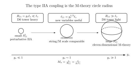
The asymptotic, dimensionless ratios $R_{11}/\ell_p=g_s^{2/3}$ and $M_{\rm KK}\ell_p=g_s^{-2/3}$ are plotted on logarithmic axes for $10^{-3}\le g_s\le10^3$. Their product is one. The crossing at $g_s=1$ compares scales; it is not a phase-transition or curvature-validity criterion. In a varying background, the local energy and curvature tests must be applied separately.

Circle reduction of an eleven-dimensional Majorana spinor gives two ten-dimensional Majorana–Weyl spinors of opposite chirality, as required by type IIA. The aligned elementary branes preserve half the supersymmetry, while their wrapping changes its ten-dimensional interpretation. The ordinary massless circle reduction does not include the Romans parameter: D8 domain walls do not enter this dictionary by the same construction. Their massive-IIA scope is a separate issue.

Exercises

Exercise 1. Gauge covariance and the signed KK source

Derive the compensating transformation of $C_3$ under $z'=z+g_s\Lambda(x)$, then obtain the horizontal field strength and its Bianchi identity. Independently eliminate the circle velocity from a massless particle action at fixed $p_z$. Explain why the mass spectrum cannot determine the sign of its D0 charge.

Solution

Invariance of $\eta$ requires $C_1'=C_1+d\Lambda$. Invariance of $\mathcal A_3$ then requires

$$C_3'=C_3-B_2\wedge d\Lambda.$$

Because $-B_2\wedge d\Lambda=\Lambda H_3-d(\Lambda B_2)$, this is equivalent modulo an RR gauge transformation to $\delta C_3=\Lambda H_3$. Direct differentiation gives

$$\delta\widetilde F_4 =-H_3\wedge d\Lambda-d\Lambda\wedge H_3=0, \qquad d\widetilde F_4=-F_2\wedge H_3.$$

The horizontal and vertical components are orthogonal in the coframe adapted to $\eta$. Four horizontal inverse metrics cancel the determinant’s factor in their norm, whereas three horizontal and one circle inverse metric leave $e^{-2\phi}$. Thus the kinetic-density factors are $g_s^2$ and $e^{-2\phi}$ as stated in the main text. Setting $g_s=1$ would hide the error made by omitting its RR factor; the equality must hold at arbitrary coupling.

For the particle, let $e$ be an einbein, $a=e^{-2\phi/3}$, $b=e^{4\phi/3}$, and $C_v=C_\mu\dot x^\mu$. Its Lagrangian and circle momentum are

$$L=\frac1{2e}\left[aG^S_{\mu\nu}\dot x^\mu\dot x^\nu +b(\dot z-g_sC_v)^2\right], \qquad p_z=\frac b e(\dot z-g_sC_v).$$

The fixed-momentum Routhian is $L_R=L-p_z\dot z$. Solving for $\dot z$ gives

$$L_R=\frac a{2e}G^S_{\mu\nu}\dot x^\mu\dot x^\nu -\frac{e\,p_z^2}{2b}-g_sp_zC_v.$$

Consequently $q=-g_sp_z$. At infinity, eliminating the einbein yields mass $|p_z|$. For $p_z=n/R_{11}$, a positive unit D0 source requires $n=-1$, since $g_s/R_{11}=1/\ell_s=\mu_0$. Both momentum signs have the same mass, which is why the mass comparison alone loses the source orientation.

Exercise 2. Wrapping, source normalization and magnetic orientation

Compute the dilaton dependence of the four wrapped/unwrapped M2 and M5 volume terms. Check their source normalizations. In the pure magnetic sector derive the circle-last component of $\mathcal A_6$ and determine the wrapped orientation that gives a positive D4.

Solution

An unwrapped $d$-dimensional worldvolume has volume factor $e^{-d\phi/3}$. If one direction wraps the circle, the factor becomes $e^{-(d-1)\phi/3+2\phi/3}=e^{-(d-3)\phi/3}$. The M2 has $d=3$ and the M5 has $d=6$, so the four factors are $e^{-\phi}$, $1$, $e^{-2\phi}$ and $e^{-\phi}$.

Using the shared lengths and tensions gives

$$\begin{aligned} T_{\rm M2}&=\frac1{(2\pi)^2g_s\ell_s^3}=T_2, &2\pi R_{11}T_{\rm M2}&=\frac1{2\pi\ell_s^2},\\ T_{\rm M5}&=\frac1{(2\pi)^5g_s^2\ell_s^6}=T_{\rm NS5}, &2\pi R_{11}T_{\rm M5}&=\frac1{(2\pi)^4g_s\ell_s^5}=T_4. \end{aligned}$$

The M2 RR term is $g_sT_{\rm M2}\int C_3=\mu_2\int C_3$; its wrapped NS term is $T_{\rm F1}\int B_2$. These coefficients test the field normalization independently of the volume terms.

For a horizontal four-form, the eleven-dimensional determinant contributes $e^{-8\phi/3}$ and the four inverse horizontal metrics contribute $e^{8\phi/3}$. With $\mathrm{vol}_{11}=\mathrm{vol}_{10}\wedge dz$ they cancel without an additional permutation sign:

$$\mathcal F_7=*_{11}(g_s\mathcal F_4^{\rm IIA}) =g_s(*_S\mathcal F_4^{\rm IIA})\wedge dz =-g_s\mathcal F_6^{\rm IIA}\wedge dz.$$

Locally, $\mathcal A_6=-g_sC_5^{\rm WZ}\wedge dz$ in this sector. Give the wrapped M5 orientation $-\omega_5\wedge dz$. Then

$$T_{\rm M5}\int_{-W_5\times S^1}\mathcal A_6 =(2\pi R_{11})g_sT_{\rm M5}\int_{W_5}C_5^{\rm WZ} =\mu_4\int_{W_5}C_5^{\rm WZ}.$$

Using the opposite wrapped orientation yields an anti-D4. For the unreversed ordering $W=\omega_5\wedge dz$, moving $dz$ past the five coordinate-normal directions gives $W\wedge(dx^5\wedge\cdots\wedge dx^9)=-\mathrm{vol}_{11}$. Its induced normal orientation is therefore opposite to the coordinate base. The actual positive-D4 source has orientation $-W$, whose induced normal orientation agrees with that base. Keeping both reversals explicit reconciles the magnetic flux with the source. This calculation is restricted to the flux-free, single-charge sector; it does not specify all M5 worldvolume couplings.

Exercise 3. Recovering the circle average and its corrections

Derive the zero mode and all nonzero Fourier coefficients of a periodic sum of $(\rho^2+z^2)^{-\nu}$. Apply the result to M2 and M5. Explain why a circle average does not commute with constructing the metric, and specify both limits needed for a local uncompactified throat.

Solution

Let $L=2\pi R_{11}$. Integrating a periodic image sum over one cell and shifting each image’s integration variable fills the real line exactly once. Its zero coefficient is

$$a_0=\frac1L\int_{-\infty}^{\infty}\frac{ds}{(\rho^2+s^2)^\nu} =\frac{\sqrt\pi\,\Gamma(\nu-\tfrac12)}{L\,\Gamma(\nu)}\rho^{1-2\nu}.$$

To obtain a nonzero coefficient, use a Schwinger parameter and perform the Gaussian integral:

$$\begin{aligned} \widehat f(k) &=\frac{\sqrt\pi}{\Gamma(\nu)}\int_0^\infty dt\,t^{\nu-3/2}e^{-\rho^2t-k^2/(4t)}\\ &=\frac{2\sqrt\pi}{\Gamma(\nu)} \left(\frac{|k|}{2\rho}\right)^{\nu-1/2}K_{\nu-1/2}(|k|\rho). \end{aligned}$$

Thus $a_n=\widehat f(n/R_{11})/L$, and the real periodic sum is $a_0+2\sum_{n\ge1}a_n\cos(nz/R_{11})$. For $\nu=3$, $a_0=3/(16R_{11}\rho^5)$; for $\nu=3/2$, $a_0=1/(\pi R_{11}\rho^2)$. Multiplying by $Q_2$ and $Q_5$ reproduces the D2 and NS5 coefficients.

At $z=0$, write $x=\rho/R_{11}$. The ratios plotted in the figure can be evaluated directly as

$$\mathcal R_2(x)=\frac{16x^5}{3}\sum_{m\in\mathbb Z}[x^2+(2\pi m)^2]^{-3}, \qquad \mathcal R_5(x)=\pi x^2\sum_{m\in\mathbb Z}[x^2+(2\pi m)^2]^{-3/2}.$$

They tend to one at large $x$. At small $x$, the central term gives $\mathcal R_2\sim16/(3x)$ and $\mathcal R_5\sim\pi/x$. The nonzero Fourier coefficients, rather than these small-$x$ approximations, determine the exponentially small large-$x$ corrections.

To see why the metric cannot simply be averaged, let $H=\overline H+\delta H$ with $\overline{\delta H}=0$. For a metric component proportional to $H^a$,

$$\overline{H^a} =(\overline H)^a \left[1+\frac{a(a-1)}2\frac{\overline{(\delta H)^2}}{(\overline H)^2}+\cdots\right].$$

The second term is generally nonzero. The smeared solution uses $\overline H$ in the nonlinear ansatz; it is not the averaged localized metric. A single-image limit requires $s_{\rm loc}\ll R_{11}$, while discarding the additive 1 additionally requires $s_{\rm loc}\ll R_2$ or $R_5$. The latter is the throat condition.

Exercise 4. Flux, coupled equations and AdS radii

Recover both harmonic coefficients from Gauss law, check the electric/magnetic charge product, and verify the relative AdS and sphere radii. Explain how the Einstein equation distinguishes an incorrect field amplitude from a reversal of its charge.

Solution

For an M2, the metric factors in the electric Hodge star cancel, leaving $-*_{8,\rm flat}dH$. Since $dH=-6Q_2r^{-7}dr$, its flux is $6\Omega_7Q_2$. The magnetic M5 field has flux $3\Omega_4Q_5$. The source equations therefore give the coefficients in the main text. Their normalization also obeys

$$2\kappa_{11}^2T_{\rm M2}T_{\rm M5} =\frac{(2\pi)^8\ell_p^9}{(2\pi)^7\ell_p^9}=2\pi.$$

The form stress is quadratic. For the M2, direct contraction produces

$$\begin{aligned} R_{\mu\nu}^{\rm form}&=-\frac{\eta_{\mu\nu}v^2}{3H^3},\\ R_{ij}^{\rm form}&=-\frac{v_iv_j}{2H^2}+\frac{\delta_{ij}v^2}{6H^2}. \end{aligned}$$

For the M5 the coefficients $1/3$ and $1/6$ in these last two terms become $1/6$ and $1/3$, respectively; the $v_iv_j$ coefficient is unchanged. Subtracting from the geometric Ricci tensor leaves only the displayed $\Delta H$ terms. Changing $\mathcal F_4\to c\mathcal F_4$ with $c^2\ne1$ spoils the cancellation at a point with $dH\ne0$. Changing its sign leaves this cancellation intact but reverses the Gauss flux. Both checks are needed.

For the M2 throat, $r^2=R_2^3/(2u)$ gives $dr/r=-du/(2u)$, producing the AdS radius $R_2/2$. For the M5, $r=4R_5^3/u^2$ gives $dr/r=-2du/u$, producing radius $2R_5$. The sphere radii remain $R_2$ and $R_5$.

An independent curvature check uses $R_{ab}=-(d-1)g_{ab}/L^2$ on AdS$_d$ and $R_{ij}=(n-1)g_{ij}/R^2$ on $S^n$. The electric M2 orthonormal flux has magnitude $6/R_2$: the eleven-dimensional equation gives $R_{ab}=-12g_{ab}/R_2^2$ and $R_{ij}=6g_{ij}/R_2^2$. The M5 orthonormal magnetic flux has magnitude $3/R_5$, giving $R_{ab}=-3g_{ab}/(2R_5^2)$ and $R_{ij}=3g_{ij}/R_5^2$. These match the two AdS radius ratios, so setting both radii equal would fail the flux-supported Einstein equations.

Exercise 5. The circle bundle and a smooth nut

Starting from the two Taub–NUT patches, calculate the first Chern number and the RR flux. Derive the near-nut period and distinguish coincident charge $N$ from $N$ separated unit centers. Track what changes for an oppositely charged source.

Solution

Both potentials differentiate to $k\sin\theta\,d\theta\wedge d\varphi$. Therefore

$$\int_{S^2}dA=4\pi k=2\pi NR_{11}, \qquad \int_{S^2}F_2=-\frac{4\pi k}{g_s}=-2\pi N\ell_s.$$

On the overlap, $(z_S-z_N)/R_{11}=N\varphi$. As $\varphi$ increases by $2\pi$, the circle transition winds $N$ times. This is the first Chern number. A formula omitting $R_{11}$ from the bundle connection would depend on the chosen length unit and cannot be a topological integer.

For $H\simeq k/r$, substitute $r=\rho_4^2/(4k)$. The radial term becomes $d\rho_4^2$, and both angular terms acquire coefficient $\rho_4^2/4$. The coordinate $\psi=z/k$ has period $2\pi R_{11}/k=4\pi/N$. Only $N=1$ has the ordinary Hopf period of a round unit three-sphere, giving a smooth origin. For coincident $N>1$ the angular space is a lens-space quotient and the origin is an orbifold point.

For separated unit centers,

$$H=1+\sum_{a=1}^N\frac{R_{11}/2}{|\mathbf r-\mathbf r_a|}.$$

Near each center the other terms are finite. The singular term has the unit coefficient, so each local nut has the smooth period, although the large linking sphere measures total charge $N$.

An antimonopole reverses $A$ and the Chern number while keeping the positive harmonic coefficient and the same metric lengths; its local Hopf orientation reverses. Replacing $N$ by a negative number inside $H=1+NR_{11}/(2r)$ would instead create a zero or negative harmonic function and would not describe that regular antibrane lift.

Exercise 6. Three independent scale questions

Derive the radius in Planck units and compare the KK and curvature tests. Give an example where a large circle still permits a zero-mode low-energy process, and explain why the D0 mass formula does not prove a single-particle state at every charge.

Solution

Since $R_{11}/\ell_p=g_s^{2/3}$,

$$\frac{R_{\rm loc}}{\ell_p} =g_s^{2/3}e^{2\phi/3}=e^{2\Phi/3}, \qquad M_{\rm KK}^{\rm loc}\ell_p=e^{-2\Phi/3}.$$

Take a locally flat circle with $R_{\rm loc}=100\ell_p$. A process with $E_{\rm loc}=10^{-4}/\ell_p$ has $E_{\rm loc}R_{\rm loc}=10^{-2}$ and cannot excite the first KK level. A process with energy $0.1/\ell_p$ does resolve it. The local curvature is zero in either case. Conversely, changing the background curvature while retaining the same circle radius can invalidate classical supergravity without changing the KK scale.

For localized M2 and M5 throats the relevant curvature radii scale as $N^{1/6}\ell_p$ and $N^{1/3}\ell_p$. Large $N$ can make the geometry weakly curved. If the circle is transverse, obtaining a local uncompactified throat further requires being close to one image, rather than merely having a large proper circle somewhere. If the circle lies along the worldvolume, its periodic identification persists even though the local metric is AdS.

Finally, $n_0$ separated positively charged D0-branes have total rest energy $n_0T_0$, the same value as a hypothetical BPS bound state. Relative motion gives a continuum beginning at this threshold. Establishing an additional normalizable state requires solving or constraining the interacting relative quantum mechanics, with care about its noncompact directions and continuum contribution. Equality of the threshold and the BPS mass supplies neither that existence argument nor a uniqueness argument. The geometric interpretation explains what the tower would represent; an index or dynamical calculation supplies independent information about which states are present.

References

• Itzhaki, Nissan, Juan M. Maldacena, Jacob Sonnenschein, and Shimon Yankielowicz. “Supergravity and the Large N Limit of Theories with Sixteen Supercharges.” Physical Review D 58 (1998), 046004. arXiv:hep-th/9802042; doi:10.1103/PhysRevD.58.046004. Sections 3, 8 and 9 discuss localized M-branes, circle averages and the D6 lift.
• Saffin, P. M. “Type IIA Killing Spinors and Calibrations.” Physical Review D 71 (2005), 025018. arXiv:hep-th/0407156; doi:10.1103/PhysRevD.71.025018. Appendix A gives the eleven-dimensional action and reduction; its fields are translated to the shared normalization here.
• Sethi, Savdeep, and Mark Stern. “D-Brane Bound States Redux.” Communications in Mathematical Physics 194 (1998), 675–705. arXiv:hep-th/9705046; doi:10.1007/s002200050374. Establishes the two-D0 threshold bound-state result by an analysis separate from the mass formula.
• Witten, Edward. “String Theory Dynamics in Various Dimensions.” Nuclear Physics B 443 (1995), 85–126. arXiv:hep-th/9503124; doi:10.1016/0550-3213(95)00158-O. Section 2 develops the relation between the IIA coupling, protected charges and an eleven-dimensional circle.