Type I Strings, Orientifolds, and Chan–Paton Factors

Type I string theory combines unoriented open and closed strings. Reversing the worldsheet orientation keeps half of the Type IIB supersymmetry, while labels attached to open-string endpoints become matrix gauge degrees of freedom. The projection determines an orthogonal or symplectic gauge algebra; consistency of the supersymmetric ten-dimensional vacuum then selects 32 endpoint labels and the algebra $\mathfrak{so}(32)$.

We will derive these statements separately, so that a state projection, a gauge-algebra calculation, and a tadpole condition each have a clear role. The setting is flat, uncompactified ten-dimensional spacetime. The shared definitions, the closed-string spectrum, and the physical vertex operators supply the conventions used below.

Type 0 projections and the closed-string alternatives

A choice of left–right GSO pairings and a projection by worldsheet orientation reversal are different operations. Type 0 strings illustrate the first operation while remaining oriented closed-string theories.

Recall that $\mathrm{NS}_+$ keeps the massless vector of one chiral sector, while $\mathrm{NS}_-$ contains its unprojected vacuum. The labels $\mathrm R_\pm$ denote eigenvalues of the total Ramond GSO grading. They coincide with the coefficient spinor’s chirality on the oscillator ground state; nonzero Ramond oscillators modify that relation.

The Type 0 sectors are

$$\begin{aligned} 0\mathrm A:\quad& (\mathrm{NS}_+,\mathrm{NS}_+)\oplus(\mathrm{NS}_-,\mathrm{NS}_-) \oplus(\mathrm R_+,\mathrm R_-)\oplus(\mathrm R_-,\mathrm R_+),\\ 0\mathrm B:\quad& (\mathrm{NS}_+,\mathrm{NS}_+)\oplus(\mathrm{NS}_-,\mathrm{NS}_-) \oplus(\mathrm R_+,\mathrm R_+)\oplus(\mathrm R_-,\mathrm R_-). \end{aligned}$$

There are no mixed NS–R sectors, hence no spacetime fermions. Level matching permits the two NS vacua to pair, giving

$$\frac{\alpha'M^2}{4}=0-\frac12, \qquad M^2=-\frac2{\alpha'}.$$

Thus the flat perturbative vacuum contains a tachyon. Both theories also have the usual massless NSNS fields $G_{\mu\nu},B_{\mu\nu},\Phi$ and twice the Type II number of RR polarizations. Type 0A has two vectors and two three-form potentials. Type 0B has two scalars, two two-form potentials, and a four-form whose five-form field strength has both dualities. Its four-form has $\binom84=70$ physical polarizations, rather than the 35 of one self-dual sector. The Type 0 calculation derives these counts. These are the spectra summarized by Angelantonj and Sagnotti, section 3.1.

Type I instead starts from supersymmetric Type IIB and gauges a symmetry that exchanges the two worldsheet orientations.

Worldsheet parity and the Type I closed spectrum

Geometrical reversal and the physical state projection

For a closed string, worldsheet parity acts by

$$\Omega:\quad (\tau,\sigma)\longmapsto(\tau,-\sigma).$$

It exchanges left and right movers. For the bosonic oscillators this means $\alpha_n^\mu\leftrightarrow\widetilde\alpha_n^\mu$. Its lift to fermions, their vacua and the ghosts must be specified consistently with interactions. A bare exchange of two raw fermion symbols does not by itself determine the parity of a physical state.

For the standard supersymmetric Type I lift, the physical projection is

$$\Pi_\Omega=\frac{1+\Omega}{2}.$$

A useful way to evaluate it is to work with the physical chiral state spaces. A massless NS factor is a spacetime boson; a massless Ramond factor is a spacetime fermion. Exchange is therefore graded: interchanging two Ramond factors contributes an additional minus sign.

In the NSNS sector, write a transverse polarization as $e_{ij}$, with $i,j=1,\ldots,8$. Then

$$\Omega:e_{ij}\longmapsto e_{ji}, \qquad \Pi_\Omega e=\frac12(e+e^{\mathsf T}).$$

The surviving symmetric tensor contains the traceless graviton and the dilaton:

$$\operatorname{Sym}^2(\mathbf8_v)=\mathbf{35}_v\oplus\mathbf1.$$

The antisymmetric $\mathbf{28}$ is the NSNS two-form and is removed.

Why the RR two-form survives

The two physical IIB Ramond factors have the same transverse chirality. In the null frame and orientation used in the RR decomposition, call this module $\mathbf8_s$. Write their tensor polarization as $M_{ab}$. Graded exchange gives

$$\Omega:M_{ab}\longmapsto-M_{ba}, \qquad \Pi_\Omega M=\frac12(M-M^{\mathsf T}).$$

The tensor product splits as

$$\mathbf8_s\otimes\mathbf8_s =\underbrace{\mathbf1\oplus\mathbf{35}_+}_{\text{symmetric}} \oplus\underbrace{\mathbf{28}}_{\text{antisymmetric}}.$$

Consequently the RR two-form $C_2$ survives, while the scalar $C_0$ and four-form potential $C_4$ do not. In IIB it is the five-form field strength of $C_4$ that is self-dual. The minus sign in RR exchange is essential: ordinary ungraded exchange would retain the wrong representations. This physical-state argument is described in Polchinski, section 3.2.

The two mixed sectors are exchanged with one another. The invariant subspace contains one vector-spinor multiplet, with 56 gravitino polarizations and eight dilatino polarizations. Gamma contraction makes the dilatino’s spinor chirality opposite to the gravitino’s, as derived on the spectrum page. In the shared IIB choice, the gravitino has ten-dimensional chirality $-1$ and the dilatino $+1$.

The result is ten-dimensional $\mathcal N=1$ supergravity:

$$N_B=35+1+28=64, \qquad N_F=56+8=64.$$

One linear combination of the two IIB supersymmetries remains, giving 16 real supersymmetry parameters.

The standard supersymmetric orientation projection keeps $G,\Phi,C_2$ and one gravitino–dilatino pair. The RR minus sign comes from exchanging two fermionic chiral factors. $C_4$ denotes a potential; its IIB field strength $F_5$ is self-dual. The labels count physical massless polarizations at nonzero null momentum, and the diagram has no geometric scale.

Crosscaps and boundaries

Gauging orientation reversal also changes the allowed worldsheet surfaces. A crosscap is an orientation-reversing identification: one may represent it by removing a disk and identifying opposite points on the resulting circle. That circle is not an ordinary open-string boundary.

At one loop the closed trace with an $\Omega$ insertion produces a Klein bottle. In the open sector, the trace without and with $\Omega$ produces an annulus and a Möbius strip. These surfaces will provide the consistency condition that fixes the open-string multiplicity. The topology is explained in Polchinski, section 1.3.

Endpoint labels and matrix wavefunctions

Give each oriented endpoint $N$ possible labels. A state at a fixed oscillator level can be written as

$$|\Psi;\lambda\rangle =\sum_{i,j=1}^N\lambda_{ij}|\Psi;i,j\rangle.$$

The coefficients form an $N\times N$ matrix, called a Chan–Paton wavefunction. Its endpoint inner product is

$$\langle\lambda_1,\lambda_2\rangle =\operatorname{tr}(\lambda_1^\dagger\lambda_2).$$

Changing the endpoint basis by a unitary matrix acts as

$$\lambda\longmapsto U\lambda U^{-1}.$$

Thus the two ends transform as $\mathbf N$ and $\overline{\mathbf N}$, and the matrix space is $\mathbf N\otimes\overline{\mathbf N}$. The massless vector is an adjoint-valued gauge field, including the central $U(1)$ before the orientation projection.

Expand the position-space field in a Hermitian basis, $A_\mu(x)=A_\mu^a(x)T^a$. This does not require each positive-momentum plane wave to be Hermitian: the reality condition relates opposite momenta,

$$A_\mu(k)^\dagger=A_\mu(-k).$$

This distinction is useful when applying the projection to complex polarization wavefunctions.

Orthogonal and symplectic endpoint projections

Consistency of applying parity twice

Reversing a string exchanges its endpoints, so it transposes $\lambda$. A unitary action on endpoint labels may accompany this transpose:

$$T_\gamma(\lambda)=\gamma\lambda^{\mathsf T}\gamma^{-1}.$$

The notation $T_\gamma$ isolates the endpoint action from the parity of the oscillator and ghost state. Applying it twice gives

$$T_\gamma^2(\lambda)=K\lambda K^{-1}, \qquad K=\gamma\gamma^{-\mathsf T}.$$

For $\Omega^2=1$ on the complete endpoint matrix algebra, $K$ must commute with every matrix and hence be proportional to the identity. Equivalently, $\gamma^{\mathsf T}=\eta\gamma$. Transposing again forces $\eta^2=1$:

$$\gamma^{\mathsf T}=\eta\gamma, \qquad \eta=+1\ \text{or}\ -1.$$

A unitary change of endpoint basis acts by congruence on $\gamma$. A symmetric unitary matrix can be brought to the identity. An antisymmetric unitary matrix can be brought to

$$J=\begin{pmatrix}0&I_n\\-I_n&0\end{pmatrix}, \qquad N=2n.$$

The evenness of $N$ is necessary: an odd-dimensional antisymmetric matrix has zero determinant and cannot be unitary. These two possibilities are derived in Polchinski, section 1.3.

The massless vector contributes a minus sign

The vector couples on the boundary through a tangential derivative. Reversing the boundary orientation reverses that tangent, so the massless vector’s worldsheet state is odd under the standard parity lift. The total state is invariant when its endpoint factor is also odd:

$$\lambda=-T_\gamma(\lambda).$$

For the superstring, this is a statement about the complete physical vector representative, including its fermion and ghost completion. The bosonic oscillator formula $\Omega\alpha_{-m}\Omega^{-1}=(-1)^m\alpha_{-m}$ gives a useful comparison, but does not fix every RNS vacuum phase. Exercise 3 makes the bosonic comparison precise.

For $\gamma=I_N$, the condition is $\lambda=-\lambda^{\mathsf T}$. A Hermitian generator satisfying it is imaginary and antisymmetric. There are

$$\dim\mathfrak{so}(N)=\frac{N(N-1)}2$$

independent generators. Their exponentials are real orthogonal matrices connected to the identity.

For $\gamma=J$, the condition becomes

$$\lambda=-J\lambda^{\mathsf T}J^{-1}.$$

Together with Hermiticity it defines the compact symplectic algebra $\mathfrak{usp}(2n)$. The finite transformations are unitary and preserve $J$, and

$$\dim\mathfrak{usp}(2n)=n(2n+1).$$

We write $\mathrm{USp}(2n)$ to display the dimension of the defining representation explicitly; it is also called $\mathrm{Sp}(n)$. Exercise 2 constructs these matrices in blocks.

Closure follows directly. Since transpose reverses multiplication,

$$T_\gamma([A,B])=-[T_\gamma(A),T_\gamma(B)].$$

If $T_\gamma(A)=-A$ and $T_\gamma(B)=-B$, then $-i[A,B]$ is both Hermitian and in the same negative eigenspace. This is the Lie bracket appropriate to the shared Hermitian generators.

The endpoint involution must be combined with the vector’s parity. Symmetric $\gamma$ gives $\mathfrak{so}(N)$; antisymmetric $\gamma$ requires $N=2n$ and gives $\mathfrak{usp}(2n)$. Both branches select the negative eigenspace of $T_\gamma$ and close under $-i[A,B]$. The diagram is algebraic and has no geometric scale.

The preserved supersymmetry relates the open NS vector and R gaugino, so the two carry the same Chan–Paton representation in the supersymmetric construction. Each surviving generator has eight vector and eight gaugino polarizations.

Disk ordering and Yang–Mills interactions

Sewing endpoint indices produces a trace

Follow the oriented boundary of a disk with $r$ open-string insertions. The endpoint label leaving one insertion is the label entering the next. Summing the internal labels gives

$$\sum_{i_1,\ldots,i_r} (\lambda_1)_{i_1i_2}(\lambda_2)_{i_2i_3}\cdots (\lambda_r)_{i_ri_1} =\operatorname{tr}(\lambda_1\lambda_2\cdots\lambda_r).$$

This explains cyclic invariance and why arbitrary permutations need not have the same color factor. Before imposing orientation identification, a convenient organization is

$$\mathcal A_r =\sum_{\sigma\in S_r/\mathbb Z_r} \operatorname{tr}(\lambda_{\sigma(1)}\cdots\lambda_{\sigma(r)}) A_r(\sigma(1),\ldots,\sigma(r)).$$

Overall coupling and external-state normalization are suppressed here. The sum already includes reversed orderings for $r>2$. One may instead organize an unoriented amplitude in reflection-related pairs, with a correspondingly adjusted overall counting; one must not add the reverse order a second time to this sum.

For surviving vector generators, the projection itself implies

$$\operatorname{tr}(\lambda_1\cdots\lambda_r) =(-1)^r\operatorname{tr}(\lambda_r\cdots\lambda_1).$$

Exercise 6 derives this relation. It matches the reversal property of the vector kinematic amplitude.

The cubic commutator

The three-vector calculation gives an ordered Yang–Mills kinematic factor $K_3$ that changes sign under reversal. At three points there are two cyclic orderings. Their sum is therefore proportional to

$$K_3\left[\operatorname{tr}(\lambda_1\lambda_2\lambda_3) -\operatorname{tr}(\lambda_1\lambda_3\lambda_2)\right] =K_3\operatorname{tr}(\lambda_1[\lambda_2,\lambda_3]).$$

For Hermitian generators with $\operatorname{tr}(T^aT^b)=\kappa\delta^{ab}$, this color factor is $i\kappa f^{bc}{}_a$. The factor of $i$ agrees with the Hermitian matrix connection: the non-Abelian term in $F_{\mu\nu}$ is $-i[A_\mu,A_\nu]$. A bare commutator would be anti-Hermitian and would not define the stated real gauge field.

The open-string vertices carry the same matrices. Using the NS supermultiplet $U_F,U_B$ already derived on the vertex page,

$$V_{-1}=\lambda\,c e^{-\phi}U_F, \qquad V_0=\lambda\,(cU_B+\gamma U_F), \qquad U_{\mathrm{int},0}=\lambda U_B.$$

The zero-picture unintegrated operator includes its superghost term. Its disappearance in a particular ghost-saturated disk correlator does not remove it from the BRST-closed vertex. Integrated and unintegrated operators have different ghost numbers.

At low energy the vector interactions begin with Yang–Mills theory. The superstring three-vector amplitude has no independent cubic-momentum term corresponding to the bosonic-string $F^3$ correction; the explicit cancellation is shown on the linked vertex page. Higher-point amplitudes do have higher-derivative corrections. In particular, a central $U(1)$ commutes with every matrix and has no Yang–Mills cubic self-coupling, while its $F^4$ interaction survives. The four-point disk expansion makes that distinction quantitative.

Why the endpoint multiplicity is 32

The orthogonal projection permits any $N$ at the level of the matrix algebra. The number 32 comes from a further consistency condition on the coupled open and closed theory.

The three closed-channel sources

Viewed in a transverse channel, the annulus describes closed-string propagation between two boundaries, the Klein bottle between two crosscaps, and the Möbius strip between a boundary and a crosscap. A long tube isolates the massless closed-string source.

Let $\epsilon=-1$ label the orthogonal vector projection and $\epsilon=+1$ the symplectic one. This sign is distinct from $\eta$ in $\gamma^{\mathsf T}=\eta\gamma$: for the vector projection, $\epsilon=-\eta$. After expressing all three amplitudes in the same closed proper time, their massless coefficients have the common normalization

$$\widetilde{\mathcal K}:\frac{2^5}{2}, \qquad \widetilde{\mathcal A}:\frac{2^{-5}N^2}{2}, \qquad \widetilde{\mathcal M}:\frac{2\epsilon N}{2}.$$

Here the NSNS and RR contributions are examined separately; a common sector-dependent exchange sign has been stripped off. The relative coefficients are the essential quantities. The annulus is quadratic in the boundary multiplicity, the Klein bottle is independent of it, and the Möbius strip supplies their interference term. The factors of two follow from modular transformations and the common proper-time measure, not from counting the massless gauge bosons. Exercise 5 derives them from the direct-channel expressions in Angelantonj and Sagnotti, equations 142–148.

Their sum is a perfect square:

$$\frac{2^5}{2}+\frac{2^{-5}N^2}{2}+\epsilon N =\frac{(N+32\epsilon)^2}{64}.$$

The unsquared expression measures the net source. For the supersymmetric orthogonal choice,

$$\epsilon=-1, \qquad N-32=0, \qquad N=32.$$

The same supersymmetric D9 setup with $\epsilon=+1$ would require $N=-32$, which is not a nonnegative endpoint multiplicity. This excludes that choice within this construction; it does not exclude symplectic gauge algebras on other branes or nonsupersymmetric orientifolds.

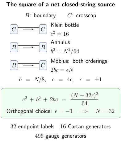
In a common transverse-channel normalization, crosscap–crosscap, boundary–boundary and boundary–crosscap exchange give the three terms in $(N+32\epsilon)^2/64$. The supersymmetric orthogonal choice has $\epsilon=-1$. The two boundary–crosscap orderings explain the interference factor two. Tubes indicate factorization channels, not metric embeddings of the original worldsheet surfaces; no geometric scale is implied.

Charge cancellation and supersymmetry

The negative-charge, negative-tension orientifold nine-plane is conventionally called an $\mathrm O9^-$ plane. D9 sources cancel its RR charge in the Type I construction. The same supersymmetric choice also cancels the NSNS tension/dilaton source.

These conditions have different meanings. An RR tadpole is an uncancelled charge source and obstructs the proposed background. A dilaton tadpole is a force on the background fields; in nonsupersymmetric examples it may remain even when the RR condition is satisfied. We are selecting the supersymmetric flat Type I vacuum, not classifying those other backgrounds.

One must therefore keep the two sectors separate before using the Jacobi identity. Supersymmetry makes the vacuum character difference $V_8-S_8$ vanish, but a cancellation between bosonic and fermionic vacuum contributions does not establish that each source vanishes.

For space-filling D9-branes, the RR charge condition can also be written using a ten-form source term proportional to

$$(N-32)\int C_{10}.$$

Varying $C_{10}$ imposes $N=32$. This top form is a constraint field with no propagating ten-dimensional massless polarization; it does not enlarge the 64-state closed bosonic spectrum. Polchinski, equation 94, gives this source interpretation. Its overall normalization depends on whether one counts branes and images separately; the endpoint multiplicity here is fixed by the displayed worldsheet coefficients.

The resulting gauge algebra has

$$N=32, \qquad \operatorname{rank}\mathfrak{so}(32)=16, \qquad \dim\mathfrak{so}(32)=496.$$

The low-energy fields are $\mathcal N=1$ supergravity coupled to a vector and Majorana–Weyl gaugino for each of these 496 generators. The phrase “SO(32) Type I” is conventional. The Chan–Paton calculation fixes the Lie algebra; the nonperturbative global form involves additional states and is $\mathrm{Spin}(32)/\mathbb Z_2$ with a particular central quotient, discussed by Witten, section 2.

Anomaly consistency and what it checks

The massless fermions are chiral, so the low-energy theory must also cancel gauge and gravitational anomalies. A useful algebraic test isolates the sixth-order gauge trace in the ten-dimensional anomaly polynomial.

For $\mathfrak{so}(N)$, the adjoint is $\Lambda^2\mathbf N$. Write $\operatorname{tr}_{f}$ for the defining-representation trace and $\operatorname{Tr}_{\mathrm{adj}}$ for the adjoint trace. The exterior-square character identity gives

$$\operatorname{Tr}_{\mathrm{adj}}F^6 =(N-32)\operatorname{tr}_{f}F^6 +15\operatorname{tr}_{f}F^2\operatorname{tr}_{f}F^4.$$

The products include exterior products of the curvature two-form; even form degree permits the characteristic-polynomial manipulation. Exercise 4 derives the identity from paired fundamental eigenvalues.

At $N=32$, the independent sixth-order single trace drops out. This is a necessary part of Green–Schwarz factorization. It does not by itself cancel the full anomaly: reducible gauge terms, mixed terms and gravitational terms must combine appropriately, and the RR two-form has the modified field strength and counterterm needed for the Green–Schwarz mechanism. The original result is Green and Schwarz’s anomaly-cancellation paper.

The dimension 496 is another useful consistency check, not an independent proof selecting this Chan–Paton construction. For example, $\mathfrak e_8\oplus\mathfrak e_8$ also has dimension $248+248=496$ and occurs in a different string construction. The worldsheet projection and the source-factorization calculation carry information that this dimension alone does not contain.

Common pitfalls

Confusing the two projections. Type 0 changes the allowed oriented closed GSO pairings. Type I gauges orientation reversal of Type IIB and requires a consistent open sector.

Keeping the symmetric RR product. The Ramond factors are fermionic. Their graded exchange makes the antisymmetric $\mathbf{28}$ invariant.

Identifying endpoint number with rank. The defining representation has dimension 32; the Cartan algebra has dimension 16. The gauge algebra itself has dimension 496.

Erasing a tadpole with a supersymmetric zero. Check NSNS and RR sources separately before setting the total vacuum character difference to zero.

Dropping the matrix convention inside an exercise. With Hermitian generators the curvature contains $-i[A_\mu,A_\nu]$, and the Hermitian Lie bracket is $-i[A,B]$.

Exercises

Exercise 1: Endpoint sewing and projected completeness

Let $\{T^a\}$ be a complete Hermitian $U(N)$ matrix basis with $\operatorname{tr}(T^aT^b)=\delta^{ab}$. Derive its completeness relation. Repeat for the imaginary antisymmetric $SO(N)$ generators, and use the result to evaluate $\sum_a\operatorname{tr}(T^aX)\operatorname{tr}(T^aY)$ for arbitrary complex matrices $X,Y$.

Solution

A complete trace-orthonormal basis gives $X=\sum_a T^a\operatorname{tr}(T^aX)$. Comparing the coefficient of an arbitrary entry of $X$ yields

$$\sum_{a\in U(N)}T^a_{ij}T^a_{kl}=\delta_{il}\delta_{jk}.$$

There is no complex conjugate on the second matrix entry in this bilinear identity. Hermiticity has already converted the Hilbert-space completeness relation into a trace pairing.

For $SO(N)$ choose

$$T^{ab}=\frac{i}{\sqrt2}(E_{ab}-E_{ba}), \qquad 1\leq a<b\leq N.$$

Their traces satisfy $\operatorname{tr}(T^{ab}T^{cd})=\delta_{ac}\delta_{bd}$ when both pairs are ordered. Summing their explicit matrix elements gives

$$\sum_{a\in SO(N)}T^a_{ij}T^a_{kl} =\frac12(\delta_{il}\delta_{jk}-\delta_{ik}\delta_{jl}).$$

Equivalently, $\sum_aT^a\operatorname{tr}(T^aX)=(X-X^{\mathsf T})/2$. Contract the completeness relation with $X_{ji}Y_{lk}$ to obtain

$$\begin{aligned} \sum_{a\in U(N)}\operatorname{tr}(T^aX)\operatorname{tr}(T^aY) &=\operatorname{tr}(XY),\\ \sum_{a\in SO(N)}\operatorname{tr}(T^aX)\operatorname{tr}(T^aY) &=\frac12\left[\operatorname{tr}(XY)-\operatorname{tr}(XY^{\mathsf T})\right]. \end{aligned}$$

The second term is part of the projected matrix propagator. It is not a license to count a reverse disk ordering twice in an amplitude whose permutation sum already contains it.

Exercise 2: Construct the compact symplectic generators

For $N=2n$, solve $A^\dagger=A$ and $A=-JA^{\mathsf T}J^{-1}$ in $n\times n$ blocks. Count the real parameters, show that $U=e^{iA}$ preserves $J$, and identify the $n=1$ algebra.

Solution

Write

$$A=\begin{pmatrix}H&B\\B^\dagger&D\end{pmatrix}, \qquad H^\dagger=H,\qquad D^\dagger=D.$$

Because $J^{-1}=-J$, direct multiplication in the projection condition gives

$$D=-H^{\mathsf T}, \qquad B=B^{\mathsf T}.$$

Thus

$$A=\begin{pmatrix}H&B\\B^\dagger&-H^{\mathsf T}\end{pmatrix}.$$

The Hermitian $H$ contains $n^2$ real parameters. The complex symmetric $B$ contains $n(n+1)$ real parameters, so the total is $n(2n+1)$.

The same condition is $AJ+JA^{\mathsf T}=0$. For $U(t)=e^{itA}$,

$$\frac{d}{dt}\left[U(t)JU(t)^{\mathsf T}\right] =iU(t)(AJ+JA^{\mathsf T})U(t)^{\mathsf T}=0.$$

At $t=0$ the expression is $J$, hence $UJU^{\mathsf T}=J$ for all $t$. Hermiticity also makes $U$ unitary. For $n=1$,

$$A=\begin{pmatrix}h&b\\b^*&-h\end{pmatrix}, \qquad h\in\mathbb R,\qquad b\in\mathbb C,$$

which is an arbitrary traceless Hermitian $2\times2$ matrix. Therefore $\mathrm{USp}(2)\simeq\mathrm{SU}(2)$.

Finally, $\det\gamma=\det\gamma^{\mathsf T}=\det(-\gamma)=(-1)^N\det\gamma$. An invertible antisymmetric $\gamma$ requires even $N$.

Exercise 3: Oscillator parity at every bosonic level

Consider the bosonic all-Neumann open string with an even oscillator vacuum and 24 transverse oscillators. Let $d_L$ be its number of oscillator states at level $L$, and let $\gamma^{\mathsf T}=\eta\gamma$. Derive the number of states after orientation projection, including the Chan–Paton factor, and evaluate it at $L=0,1,2$.

Solution

The cosine modes obey $\cos[m(\pi-\sigma)]=(-1)^m\cos(m\sigma)$, so $\Omega\alpha_{-m}\Omega^{-1}=(-1)^m\alpha_{-m}$. A state with occupations $N_m$ has

$$\Omega_{\rm osc}=(-1)^{\sum_m mN_m}=(-1)^L.$$

On the $N^2$-dimensional matrix space,

$$\operatorname{Tr}T_\gamma =\sum_{ij}\gamma_{ij}(\gamma^{-1})_{ij} =\operatorname{tr}(\gamma\gamma^{-\mathsf T})=\eta N.$$

Take the trace of the full projector $(1+\Omega_{\rm osc}T_\gamma)/2$ at level $L$:

$$D_L=\frac{d_L}{2}\left[N^2+\eta(-1)^L N\right].$$

The transverse partition function is $\prod_{m\geq1}(1-q^m)^{-24}$. Its first coefficients can also be counted directly:

$$\begin{aligned} d_0&=1,\\ d_1&=24,\\ d_2&=24+\frac{24\cdot25}{2}=324. \end{aligned}$$

At level two, the first term counts one $\alpha_{-2}$ and the second two commuting $\alpha_{-1}$ oscillators. Therefore

$$D_0=\frac{N(N+\eta)}2, \qquad D_1=24\frac{N(N-\eta)}2, \qquad D_2=324\frac{N(N+\eta)}2.$$

For the orthogonal choice $\eta=+1$, the vector level uses antisymmetric matrices, while the vacuum and level two use symmetric matrices. This is a bosonic-string comparison. Its vacuum tachyon is not a state of supersymmetric Type I, and the formula does not replace the RNS fermion, spin-vacuum and ghost parity analysis.

Exercise 4: The sixth-order adjoint trace

Use the defining representation of $SO(N)$ to derive the quadratic, quartic and sixth-order adjoint trace identities. Explain precisely what the sixth-order identity establishes at $N=32$.

Solution

Let $x_i$ be the formal eigenvalues of a Cartan-valued curvature. They occur in opposite pairs, with an additional zero for odd $N$. Set $p_{2k}=\sum_i x_i^{2k}=\operatorname{tr}_fF^{2k}$. The defining character is

$$\chi_f(t)=N+\frac{t^2}{2}p_2+\frac{t^4}{24}p_4+\frac{t^6}{720}p_6+O(t^8).$$

The eigenvalues on $\Lambda^2\mathbf N$ are $x_i+x_j$ with $i<j$. Thus

$$\chi_{\mathrm{adj}}(t) =\sum_{i<j}e^{t(x_i+x_j)} =\frac12\left[\chi_f(t)^2-\chi_f(2t)\right].$$

The subtraction removes the terms with identical indices. Expanding and multiplying each coefficient by its factorial gives

$$\begin{aligned} \operatorname{Tr}_{\mathrm{adj}}F^2&=(N-2)p_2,\\ \operatorname{Tr}_{\mathrm{adj}}F^4&=(N-8)p_4+3p_2^2,\\ \operatorname{Tr}_{\mathrm{adj}}F^6&=(N-32)p_6+15p_2p_4. \end{aligned}$$

For example, the mixed sixth-order term comes from

$$\frac12\,2\left(\frac{p_2t^2}{2}\right) \left(\frac{p_4t^4}{24}\right) =\frac{p_2p_4t^6}{48},$$

and $6!/48=15$. At $N=32$, only the reducible product remains. This eliminates the independent sixth-order single trace in the adjoint gaugino contribution, but does not calculate the full anomaly polynomial or its Green–Schwarz counterterm.

For comparison, the adjoint of $\mathrm{USp}(N)$, with even $N$, is the symmetric square of its defining representation. Replacing the subtraction by addition gives $(N+32)p_6+15p_2p_4$. There is no positive $N$ that removes this coefficient in the same supersymmetric adjoint-fermion comparison. Nonsupersymmetric symplectic string models have a different fermion spectrum, so this calculation does not classify them.

Exercise 5: Derive the transverse coefficients

Write $Z(\tau)=(V_8-S_8)(\tau)/\eta(\tau)^8$ as a formal spin-structure combination. Retain the separate character coefficients throughout the modular transformation and the extraction of NSNS and RR sources; do not first replace the combination by its vanishing numerical value. The direct-channel expressions, with a common normalization suppressed, are

$$\begin{aligned} \mathcal K&=\frac12\int_0^\infty\frac{dt}{t^6}Z(2it),\\ \mathcal A&=\frac{N^2}{2}\int_0^\infty\frac{dt}{t^6}Z(it/2),\\ \mathcal M&=\frac{\epsilon N}{2}\int_0^\infty\frac{dt}{t^6}\widehat Z(1/2+it/2). \end{aligned}$$

Use the modular laws

$$Z(iu)=u^4Z(i/u), \qquad \widehat Z(1/2+it/2)=t^4\widehat Z(1/2+i/(2t))$$

to derive the three coefficients in a common transverse variable $\ell$. Hats specify the standard phase-adjusted Möbius characters; the second law is the corresponding $P$ transformation. These transformation laws are supplied inputs for the formal combinations. The $S$ transformation mixes individual characters, so the first law is not a separate transformation law for $V_8/\eta^8$ and $S_8/\eta^8$. Explain the source condition obtained from their sum.

Solution

For the Klein bottle, set $\ell=1/(2t)$. Reversing the integration limits removes the sign of $dt$, and

$$\left|\frac{dt}{t^6}\right|=32\ell^4d\ell, \qquad Z(2it)=\ell^{-4}Z(i\ell).$$

This gives $\widetilde{\mathcal K}=16\int d\ell\,Z(i\ell)$.

For the annulus, set $\ell=2/t$. Now

$$\left|\frac{dt}{t^6}\right|=\frac{\ell^4}{32}d\ell, \qquad Z(it/2)=\ell^{-4}Z(i\ell),$$

so $\widetilde{\mathcal A}=N^2\int d\ell\,Z(i\ell)/64$.

For the Möbius strip use $\ell=1/(2t)$ again. The Jacobian is the Klein-bottle one, but the hatted transformation contributes $t^4=1/(16\ell^4)$. Therefore

$$\widetilde{\mathcal M} =\epsilon N\int_0^\infty d\ell\, \widehat Z(1/2+i\ell).$$

The long-tube massless coefficients add to

$$16+\frac{N^2}{64}+\epsilon N =\left(\frac{N}{8}+4\epsilon\right)^2.$$

This is the square of a net source: a boundary contribution proportional to $N/8$ and a crosscap contribution proportional to $4\epsilon$. Only the relative normalization has been fixed. For $\epsilon=-1$, neutrality gives $N=32$; for $\epsilon=+1$ there is no nonnegative solution in this supersymmetric construction.

The RR source is linear before exchange squares it. Equivalently, variation of a source term proportional to $(N-32)\int C_{10}$ enforces neutrality. A ten-form has no propagating polarization in ten dimensions. Setting $V_8-S_8=0$ at the outset would conceal this charge constraint behind a cancellation of total vacuum contributions. The calculation derived the Jacobians and coefficient square from the supplied modular laws; it did not derive those laws from the theta functions.

Exercise 6: Color reflection and the Hermitian connection

For the surviving vector matrices, derive trace reversal and the cubic commutator. Starting from $D'_\mu=UD_\mu U^{-1}$, derive the gauge transformation of $A_\mu$ and show that its curvature transforms covariantly. Finally, explain why the vanishing central cubic coupling does not force every central quartic color factor to vanish.

Solution

Every vector matrix obeys $\lambda_i=-\gamma\lambda_i^{\mathsf T}\gamma^{-1}$. Insert this into the ordered product and cancel adjacent $\gamma^{-1}\gamma$ factors:

$$\operatorname{tr}(\lambda_1\cdots\lambda_r) =(-1)^r\operatorname{tr}(\lambda_1^{\mathsf T}\cdots\lambda_r^{\mathsf T}) =(-1)^r\operatorname{tr}(\lambda_r\cdots\lambda_1).$$

At three points, the reversed kinematic factor also has a minus sign. Combining the two cyclic orderings gives $K_3\operatorname{tr}(\lambda_1[\lambda_2,\lambda_3])$. The trace identity and the kinematic identity explain why the two full contributions agree; they do not generate two additional orderings.

Apply the transformed derivative to a test vector. Since $U(\partial_\mu U^{-1})=-(\partial_\mu U)U^{-1}$,

$$D'_\mu=\partial_\mu-iA'_\mu, \qquad A'_\mu=UA_\mu U^{-1}-i(\partial_\mu U)U^{-1}.$$

For unitary $U$, $(\partial_\mu U)U^{-1}$ is anti-Hermitian, so the last term is Hermitian. Taking commutators gives

$$[D'_\mu,D'_\nu] =U[D_\mu,D_\nu]U^{-1} =-iUF_{\mu\nu}U^{-1}, \qquad F'_{\mu\nu}=UF_{\mu\nu}U^{-1}.$$

Expanding the original commutator recovers the shared curvature with $-i[A_\mu,A_\nu]$. Its derivative terms and commutator term are all Hermitian.

For a central generator $T^0=I_N/\sqrt N$, the cubic factor $\operatorname{tr}(T^0[T^a,T^b])$ vanishes by cyclicity. Nevertheless,

$$\operatorname{tr}[(T^0)^4]=\frac1N\ne0.$$

This identity-matrix example concerns the unprojected $U(N)$ theory; the identity is not a generator of $\mathfrak{so}(32)$ or $\mathfrak{usp}(2n)$. Other Abelian Cartan directions can also have nonzero quartic traces. A nonzero trace alone does not prove that a complete amplitude is nonzero; the actual disk four-point expansion supplies the kinematic result and its Abelian $F^4$ interaction.

References

• Angelantonj, Carlo, and Augusto Sagnotti. “Open Strings.” Physics Reports 371 (2002): 1–150; erratum 376 (2003): 407. arXiv:hep-th/0204089. Sections 3.1–3.2 give the Type 0 and Type I constructions; equations 142–148 give the direct and transverse amplitudes. Their orientifold-plane superscripts use a different naming convention; the physical charge and tension signs determine the translation.
• Green, Michael B., and John H. Schwarz. “Anomaly Cancellations in Supersymmetric D=10 Gauge Theory and Superstring Theory.” Physics Letters B 149 (1984): 117–122. doi:10.1016/0370-2693(84)91565-X.
• Polchinski, Joseph. “TASI Lectures on D-Branes.” In Fields, Strings and Duality, edited by Costas Efthimiou and Brian Greene, 293–356. World Scientific, 1997. arXiv:hep-th/9611050. Sections 1.2–1.3 derive Chan–Paton factors and parity; sections 3.2 and 3.5 discuss the Type I spectrum and RR source cancellation.
• Witten, Edward. “D-Branes and K-Theory.” Journal of High Energy Physics 12 (1998): 019. doi:10.1088/1126-6708/1998/12/019, arXiv:hep-th/9810188. Section 2 explains why the global gauge group requires nonperturbative information.