Massless Closed-String Vertices and Gauge Invariance

A closed string at its first excited level carries a tensor polarization. Its two indices do not describe an arbitrary spacetime tensor: the stress-tensor OPE imposes transversality, and gauge equivalence removes the remaining longitudinal directions. The physical tensor then separates into a graviton, an antisymmetric two-form, and a scalar dilaton. This page derives that separation and explains how the same gauge redundancy appears as BRST exactness and as a worldsheet total derivative.

The setting is the flat critical bosonic string with nonzero real null momentum, no winding, and one timelike target coordinate. Formulas with a symbolic $D$ describe the tensor algebra; the uncompactified quantum theory considered here has $D=26$. We use the global conventions, the state–operator map, and the BRST transformations. The bosonic vacuum is tachyonic; identifying its massless states does not establish vacuum stability.

Massless tensor vertices and their stress poles

The matter state at $N=\widetilde N=1$ is

$$|E;k\rangle=E_{\mu\nu}\alpha_{-1}^\mu \widetilde\alpha_{-1}^\nu|0;k\rangle.$$

It is useful to distinguish the simple tensor composite from its exact oscillator normalization:

$$V_E=E_{\mu\nu}:\partial X^\mu\bar\partial X^\nu e^{ik\cdot X}:, \qquad \mathcal U_E=-\frac2{\alpha'}V_E \ \longleftrightarrow\ |E;k\rangle.$$

The coefficient follows from applying $i\sqrt{2/\alpha'}\,\partial X$ once in each sector. The colons enclose the entire product: derivatives and the exponential at the same point must be jointly normal ordered. An overall rescaling does not affect the primary test, but matters when comparing a two-point coefficient with an oscillator norm.

For an allowed matter operator, the integrated insertion is $\int d^2z\,\mathcal U_E$ and the fixed insertion is $c\widetilde c\,\mathcal U_E$. The latter has weights $(0,0)$ if the matter field is a $(1,1)$ primary. The general vertex construction is discussed by Tong, §5.4.1; here we will also keep track of the gauge quotient.

Why the double pole is not the whole test

Let $h_k=\alpha'k^2/4$ be the holomorphic weight of the exponential. Adding one holomorphic derivative gives a double-pole coefficient $1+h_k$. But a primary must have no pole above order two. To find the potential third pole, contract one of the two derivatives in $T$ with the derivative in $V_E$, and the other with the exponential. There are two assignments:

$$-\frac2{\alpha'} \left(-\frac{\alpha'}{2}\frac{\eta^{\rho\mu}}{(z-w)^2}\right) \left(-\frac{i\alpha'}{2}\frac{k_\rho}{z-w}\right) =-\frac{i\alpha'}{2}\frac{k^\mu}{(z-w)^3}.$$

The uncontracted antiholomorphic derivative remains in the answer. The other contractions give the double pole and, after Taylor expansion, the translation term:

$$\begin{aligned} T(z)V_E(w,\bar w)\sim{}& -\frac{i\alpha' k^\mu E_{\mu\nu}}{2(z-w)^3} :\bar\partial X^\nu e^{ik\cdot X}:\\ &+\frac{(1+h_k)V_E(w,\bar w)}{(z-w)^2} +\frac{\partial V_E(w,\bar w)}{z-w}. \end{aligned}$$

The corresponding barred third pole is

$$-\frac{i\alpha' E_{\mu\nu}k^\nu}{2(\bar z-\bar w)^3} :\partial X^\mu e^{ik\cdot X}:.$$

These are separated-point OPEs. Mixed holomorphic–antiholomorphic contractions have contact support; they are not extra holomorphic poles. The joint composite and any integrated correlator must treat those contact terms consistently, as explained on page 10.

Thus, for a nonzero tensor operator, the $(1,1)$ primary conditions are

$$k^2=0, \qquad k^\mu E_{\mu\nu}=0, \qquad E_{\mu\nu}k^\nu=0.$$

The first condition fixes the mass; the other two constrain different indices. In oscillator language they are the two $L_0$ conditions and the independent $L_1,\widetilde L_1$ constraints. Higher positive modes annihilate this level automatically.

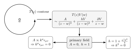
The two contractions refer to field slots in the holomorphic stress tensor, not to distinct target directions. Together they give the cubic coefficient $-i\alpha'k^\mu E_{\mu\nu}/2$ for the unscaled composite $V_E$. The barred stress tensor tests the other index. Contraction lines are schematic and carry no spacetime length scale.

Transverse constraints still leave gauge directions

A tensor of the form $k_\mu\xi_\nu$ passes both constraints if $k^2=0$ and $k\cdot\xi=0$. Its pairing with any constrained tensor vanishes. It is therefore not a new positive-norm particle polarization. The physical equivalence is

$$E_{\mu\nu}\sim E_{\mu\nu} +k_\mu\xi_\nu+\widetilde\xi_\mu k_\nu, \qquad k\cdot\xi=k\cdot\widetilde\xi=0.$$

The restrictions on the parameters are essential within this transverse on-shell description. For example,

$$k^\mu\delta E_{\mu\nu}=(k\cdot\widetilde\xi)k_\nu, \qquad \delta E_{\mu\nu}k^\nu=(k\cdot\xi)k_\mu.$$

Arbitrary spacetime gauge transformations exist before imposing a gauge; they need not preserve this particular representative. The null-state derivation and its relation to physical pairings are given by Polchinski, §2.3 and on page 7.

For nonzero null $k$, each constrained index lies in a $(D-1)$-dimensional space. The tensor space therefore has dimension $(D-1)^2$. The two transverse gauge parameters contain $2(D-1)$ components, but

$$(\xi,\widetilde\xi)\longmapsto (\xi+a k,\widetilde\xi-a k)$$

does not change $\delta E$. Conversely, this is the entire parameter kernel at nonzero $k$. The gauge image has dimension $2D-3$, leaving

$$(D-1)^2-(2D-3)=(D-2)^2$$

physical polarizations. At $D=26$ this is $625-49=576$. Primarity alone would retain the 49 null directions. At exactly $k=0$ these rank arguments fail: the constraints and the displayed gauge image both collapse. Exceptional zero-momentum states require a separate cohomology analysis.

Selecting a covariant transverse representative

Choose a null reference vector $\ell$ with $k\cdot\ell=-1$. It exists for every nonzero real null $k$. The tensor

$$P_{\mu\nu}=\eta_{\mu\nu}+k_\mu\ell_\nu+\ell_\mu k_\nu$$

annihilates $k$ and $\ell$. With one index raised it satisfies

$$P_\mu{}^\rho P_{\rho\nu}=P_{\mu\nu}, \qquad \operatorname{tr}P=D-2\equiv d.$$

To see its geometric meaning, decompose any vector as

$$v^\mu=(Pv)^\mu-k^\mu(\ell\cdot v)-\ell^\mu(k\cdot v).$$

The first term is orthogonal to both null vectors. Their longitudinal plane has one timelike and one spacelike direction, so its orthogonal complement is Euclidean. $P$ is the identity on that $d$-dimensional physical transverse space.

For a constrained tensor, act on both indices:

$$E^\perp_{\mu\nu}=P_\mu{}^\rho P_\nu{}^\sigma E_{\rho\sigma}.$$

Terms containing $k^\rho E_{\rho\sigma}$ or $E_{\rho\sigma}k^\sigma$ vanish, leaving

$$\begin{aligned} E^\perp_{\mu\nu}-E_{\mu\nu}={}& k_\mu\ell^\rho E_{\rho\nu} +k_\nu E_{\mu\sigma}\ell^\sigma\\ &+k_\mu k_\nu\ell^\rho E_{\rho\sigma}\ell^\sigma. \end{aligned}$$

Each term has a longitudinal index, and the accompanying parameter is transverse to $k$. Projection therefore changes only the gauge representative. It does not discard a physical mode. Changing $\ell$ makes another such choice; exercise 3 proves reference independence for a general tensor.

Graviton, two-form and scalar

In an orthonormal transverse basis, write $t=\delta^{ij}E^\perp_{ij}$. The three orthogonal pieces are

$$\begin{aligned} E^\perp_{ij}&=h^G_{ij}+b_{ij}+\frac{t}{d}\delta_{ij},\\ h^G_{ij}&=E^\perp_{(ij)}-\frac{t}{d}\delta_{ij}, \qquad b_{ij}=E^\perp_{[ij]}. \end{aligned}$$

The symmetric traceless tensor is the graviton polarization, the antisymmetric tensor is the two-form polarization, and the transverse trace is the scalar dilaton polarization. These are representations of the rotation part $SO(D-2)$ of the massless little group. The translation part acts trivially on the ordinary physical quotient.

Their dimensions are

$$\dim G=\frac{d(d+1)}2-1, \qquad \dim B=\frac{d(d-1)}2, \qquad \dim\Phi=1.$$

At $d=24$ they give $299+276+1=576$. This is a decomposition of the entire massless level. A particular amplitude may couple to fewer pieces: two tachyons have a symmetric tensor current, so their massless exchange contains the graviton and dilaton but no antisymmetric tensor, as derived on page 21.

A unit scalar representative is

$$E^{(\Phi)}_{\mu\nu}=\frac{P_{\mu\nu}}{\sqrt d}, \qquad E^{(\Phi)}_{\mu\nu}E^{(\Phi)\mu\nu}=1.$$

Indeed, its squared norm is $\operatorname{tr}P^2/d=1$. The tempting replacement $E_{\mu\nu}\propto\eta_{\mu\nu}$ would fail the primary test because $k^\mu\eta_{\mu\nu}=k_\nu\ne0$. The subtraction must use the rank-$d$ transverse metric, not a trace subtraction in all $D$ directions.

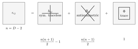
The four-dimensional illustration uses $k=E(1,0,0,1)$ and $\ell=(1,0,0,-1)/(2E)$, giving $P_{\mu\nu}=\operatorname{diag}(0,1,1,0)$. The longitudinal panel shows the dimensionless vectors $k/E$ and $E\ell$; their orthogonality relations use the Minkowski metric. The transverse plane is Euclidean. This illustrates the quotient geometry, not a four-dimensional uncompactified critical bosonic string; the general transverse rank is $d=D-2$.

From polarization shifts to spacetime gauge symmetry

Let $S_{\mu\nu}=E_{(\mu\nu)}$ and $A_{\mu\nu}=E_{[\mu\nu]}$. Introduce the combinations

$$\lambda_\mu=\frac{\xi_\mu+\widetilde\xi_\mu}{2}, \qquad \rho_\mu=\frac{\xi_\mu-\widetilde\xi_\mu}{2}.$$

Their variations are

$$\delta S_{\mu\nu}=k_\mu\lambda_\nu+k_\nu\lambda_\mu, \qquad \delta A_{\mu\nu}=k_\mu\rho_\nu-k_\nu\rho_\mu.$$

For a spacetime plane wave $e^{ik\cdot x}$, differentiation introduces $ik_\mu$. Thus choosing Fourier amplitudes $\zeta=-i\lambda$ and $\Lambda=-i\rho$ gives the familiar linearized transformations

$$\delta h_{\mu\nu}=\partial_\mu\zeta_\nu+\partial_\nu\zeta_\mu, \qquad \delta B_{\mu\nu}=\partial_\mu\Lambda_\nu-\partial_\nu\Lambda_\mu.$$

An overall conversion between a vertex polarization and a spacetime field rescales its gauge parameter as well. The two-form transformation is reducible: $\Lambda\to\Lambda+d\omega$ has no effect on $B$. Its gauge-invariant local field strength is

$$H=dB, \qquad H_{\mu\nu\rho}=\partial_\mu B_{\nu\rho} +\partial_\nu B_{\rho\mu}+\partial_\rho B_{\mu\nu}.$$

Since $d^2=0$, $\delta H=0$. The free two-form equation is $\partial^\mu H_{\mu\nu\rho}=0$; in transverse gauge it reduces to $\Box B_{\nu\rho}=0$. These local statements do not imply that every closed two-form is globally exact on an arbitrary target.

The scalar is not an extra Einstein graviton trace

For a metric perturbation, de Donder gauge is

$$\partial^\mu\left(h_{\mu\nu}-\frac12\eta_{\mu\nu}h\right)=0, \qquad h=\eta^{\mu\nu}h_{\mu\nu}.$$

It becomes $\partial^\mu h_{\mu\nu}=0$ after selecting a traceless graviton. Applying that shortened condition indiscriminately to the scalar would mix two different fields.

A useful bridge uses the leading linearized spacetime equations. These are additional low-energy input, developed on page 23, rather than a nonlinear consequence proved by the flat-worldsheet OPE. Around constant $\Phi_\infty$ and flat metric, their relevant form is

$$R^{(1)}_{\mu\nu}(h^S)+2\partial_\mu\partial_\nu\phi=0, \qquad \Box\phi=0.$$

Here $h^S$ is the string-frame metric perturbation and $\phi=\Phi-\Phi_\infty$ is the dimensionless dilaton fluctuation. These equations and the field redefinition are discussed by Polchinski, §3.1, and Tong, §§7.2.3–7.3.1. For a transverse plane-wave metric amplitude of trace $t$, the Ricci tensor is $t k_\mu k_\nu/2$. At nonzero null momentum the first equation fixes the scalar amplitude to $t/4$.

The Einstein-frame redefinition, normalized to leave the background metric unchanged, gives at linear order

$$G^E=e^{-4\phi/d}G^S, \qquad h^E_{\mu\nu}=h^S_{\mu\nu}-\frac{4\phi}{d}\eta_{\mu\nu}.$$

For plane-wave amplitudes, write $\phi(x)=\phi_k e^{ik\cdot x}$ and insert $\phi_k=t/4$ and $\eta=P-k\ell-\ell k$:

$$h^E_{\mu\nu} =\underbrace{\left(h^S_{\mu\nu}-\frac{t}{d}P_{\mu\nu}\right)}_{h^G_{\mu\nu}} +\frac{t}{d}(k_\mu\ell_\nu+\ell_\mu k_\nu).$$

The first term is transverse and traceless. The second is pure gauge. In particular, a pure transverse trace has no physical Einstein graviton, but does have a scalar fluctuation. Exercise 4 verifies the Ricci and gauge statements explicitly.

This relation uses $h^S$ as a metric amplitude; it does not determine the overall canonical normalization relating that field to $\mathcal U_E$. Nor may one set $k=0$ inside the null-reference construction to obtain the constant-dilaton coupling. That sector involves the curved-worldsheet completion and the topology weight, treated on the next page.

Longitudinal vertices, BRST exactness and contact terms

For transverse parameters, define two jointly ordered matter fields

$$\mathcal A=:\xi\cdot\bar\partial X e^{ik\cdot X}:, \qquad \mathcal B=:\widetilde\xi\cdot\partial X e^{ik\cdot X}:.$$

They are primaries of weights $(0,1)$ and $(1,0)$, respectively. At separated insertions, the free equation $\partial\bar\partial X=0$ and differentiation of the exponential give

$$\delta V_E=-i\partial\mathcal A-i\bar\partial\mathcal B.$$

There are two related interpretations, with different scopes.

First, in the critical matter-plus-ghost theory let $s$ be the graded action of the total left-plus-right BRST charge. Its local transformations imply

$$\begin{aligned} s(\widetilde c\,\mathcal A)&=c\widetilde c\,\partial\mathcal A,\\ s(c\,\mathcal B)&=-c\widetilde c\,\bar\partial\mathcal B. \end{aligned}$$

Consequently,

$$c\widetilde c\,\delta V_E =s\bigl(-i\widetilde c\,\mathcal A+i c\,\mathcal B\bigr).$$

The fixed longitudinal vertex is BRST exact. The gauge parameter has ghost number one and total weights $(0,0)$; the vertex has ghost number two. The relative sign is a Grassmann sign, not an arbitrary polarization convention. Exercise 1 supplies the full product-rule calculation. For $\mathcal U_E$, multiply the vertex and gauge parameter by $-2/\alpha'$.

Second, the local integrated variation is an exterior derivative. In the shared complex measure,

$$d^2z\,\delta V_E=d\Omega, \qquad \Omega=\mathcal A\,d\bar z-\mathcal B\,dz.$$

For a smooth, globally defined one-form on a compact surface without boundary, its integral is zero. A scattering correlator has operator insertions, however. Remove small disks around those punctures before applying Stokes: the resulting domain has boundaries, even when the underlying surface is a sphere. Contact distributions may remain when the disks shrink. A plane chart also requires control of infinity.

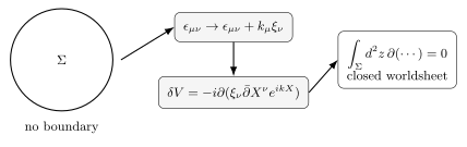
The illustrative annulus has dimensionless coordinate radii $\epsilon=1/4$ and $R=1$, drawn with equal real and imaginary scales. Its induced boundary orientation is outer counterclockwise and inner clockwise. Stokes applies to the sum of both contours. These are coordinate and puncture cutoffs, not physical boundaries of a closed string; the complementary infinity chart must also be included on a sphere. For $F=|z|^{2a}/\bar z$, the local diagnostic is $\int d^2z\,\partial F=2\pi(R^{2a}-\epsilon^{2a})$.

In a full amplitude, moving the BRST contour also encounters the antighost insertions that integrate over moduli. Their BRST variations insert the stress tensor, producing total derivatives in moduli space. The decoupling theorem therefore requires a consistent treatment of contact terms and degeneration boundaries, usually established in a suitable convergence region and then continued analytically. Polchinski, the end of §2.8, explains this additional step. The local exactness calculation is essential, but does not alone justify throwing away every boundary term. Pages 18 and 21 describe the moduli and degeneration ingredients.

Common pitfalls

Correct weights do not guarantee a primary. The tensor’s double poles give $(1,1)$ when $k^2=0$, but the third poles test its polarization. Even after these vanish, longitudinal BRST-exact states remain.

A scalar trace must be transverse. The physical scalar uses $P/\sqrt{D-2}$. A bare $\eta_{\mu\nu}$ is not transverse, and the traceful string-frame metric is not an additional Einstein graviton polarization.

A total derivative need not have a vanishing regulated integral. Puncture circles, contact terms and moduli boundaries are part of the calculation. Topological closedness of the original surface does not remove them individually.

Exercises

1. Construct the closed-string BRST gauge parameter

Derive the two BRST product identities used above. Keep the fixed ghost order $c\widetilde c$, explain the weights and ghost numbers, and determine what fails if $k\cdot\xi\ne0$.

Solution

For even matter primaries of the stated weights,

$$\begin{aligned} s\mathcal A&=c\partial\mathcal A +\widetilde c\bar\partial\mathcal A +(\bar\partial\widetilde c)\mathcal A,\\ s\mathcal B&=c\partial\mathcal B+(\partial c)\mathcal B +\widetilde c\bar\partial\mathcal B. \end{aligned}$$

Also $sc=c\partial c$ and $s\widetilde c=\widetilde c\bar\partial\widetilde c$. Because each ghost is odd, the product rule gives

$$\begin{aligned} s(\widetilde c\mathcal A) &=\widetilde c\bar\partial\widetilde c\,\mathcal A -\widetilde c\bigl[c\partial\mathcal A +(\bar\partial\widetilde c)\mathcal A\bigr]\\ &=c\widetilde c\partial\mathcal A,\\ s(c\mathcal B) &=c\partial c\,\mathcal B -c\bigl[(\partial c)\mathcal B +\widetilde c\bar\partial\mathcal B\bigr]\\ &=-c\widetilde c\bar\partial\mathcal B. \end{aligned}$$

Terms proportional to a square of the same ghost vanish. In the first identity the last step also uses $\widetilde c c=-c\widetilde c$. Multiplication by $-i$ and $+i$ produces exactly $c\widetilde c\delta V_E$.

The ghost cancels the nonzero matter weight in each seed, so both $\widetilde c\mathcal A$ and $c\mathcal B$ have weights $(0,0)$ and ghost number one. A nonzero exact operator is still a closed operator, since the critical BRST charge is nilpotent; closure is not a test that its cohomology class is nonzero.

If $k\cdot\xi\ne0$, $\mathcal A$ has a barred third stress pole with coefficient

$$\mathcal C=-\frac{i\alpha'}2(k\cdot\xi):e^{ik\cdot X}:.$$

Its BRST variation then includes $\tfrac12(\bar\partial^2\widetilde c)\mathcal C$. The first product identity acquires $-\tfrac12\widetilde c\bar\partial^2\widetilde c\,\mathcal C$. The variation is no longer just the desired tensor vertex. Consistently, $k_\mu\xi_\nu$ fails right transversality. Gauge transformations before gauge fixing still exist, but their representation cannot be restricted to the same transverse tensor ansatz without these extra terms.

2. Derive the physical polarization sums

Construct the projectors onto the graviton, two-form and scalar using $P$. Prove their orthogonality, completeness and dimensions. Recover the oscillator norm from a separated-point two-point function of $\mathcal U_E$.

Solution

Use the target metric to raise the contracted indices in products. The three kernels with lower indices are

$$\begin{aligned} \Pi^G_{\mu\nu,\rho\sigma} &=\frac12(P_{\mu\rho}P_{\nu\sigma}+P_{\mu\sigma}P_{\nu\rho}) -\frac1dP_{\mu\nu}P_{\rho\sigma},\\ \Pi^B_{\mu\nu,\rho\sigma} &=\frac12(P_{\mu\rho}P_{\nu\sigma}-P_{\mu\sigma}P_{\nu\rho}),\\ \Pi^\Phi_{\mu\nu,\rho\sigma} &=\frac1dP_{\mu\nu}P_{\rho\sigma}. \end{aligned}$$

After projecting to the transverse space these act on a matrix $M$ as $M_{(ij)}-\delta_{ij}\operatorname{tr}M/d$, $M_{[ij]}$, and $\delta_{ij}\operatorname{tr}M/d$. Repeating an operation changes nothing. Applying a different operation gives zero, because an antisymmetric tensor has no trace and the symmetric traceless part is orthogonal to the identity. Therefore

$$\Pi^A\Pi^B=\delta^{AB}\Pi^A, \qquad \Pi^G+\Pi^B+\Pi^\Phi=P\otimes P,$$

where the repeated label $A$ on the right is not summed. The symmetric and antisymmetric subspaces have dimensions $d(d+1)/2$ and $d(d-1)/2$; removing or retaining their single trace gives the claimed ranks. These arguments use the positive transverse inner product, not an unrestricted Lorentzian tensor space.

For transverse tensors at opposite null momenta, derivative–exponential cross-contractions vanish. The one holomorphic and one antiholomorphic derivative contraction give

$$\begin{aligned} \langle\mathcal U_{E^*}(-k;z,\bar z)\mathcal U_E(k;0)\rangle_{\rm stripped} &=\frac4{\alpha'^2}\frac{\alpha'^2}{4|z|^4} E^*_{\mu\nu}E^{\mu\nu}\\ &=\frac{\sum_{ij}|E^\perp_{ij}|^2}{|z|^4}. \end{aligned}$$

The momentum delta function is stripped and the vacuum pairing normalized to one. Thus the unit scalar has coefficient one, as do normalized ST and antisymmetric polarizations. Gauge directions pair to zero with every constrained tensor.

Using $D$ instead of $d$ in the trace subtraction fails an actual projector test. Applied to $P$, the supposed traceless map would give $(1-d/D)P=2P/D$, which still has nonzero trace and is not annihilated by a second trace projection.

3. Make a finite change of null reference

Let $a\cdot k=a\cdot\ell=0$ and define $\ell'=\ell+a+(a^2/2)k$. Show that it is another allowed reference. For a general constrained tensor, compare its two projected representatives and their pairing with an arbitrary constrained test tensor.

Solution

Since $k^2=\ell^2=0$ and $k\cdot\ell=-1$,

$$k\cdot\ell'=-1, \qquad \ell'^2=a^2+a^2(k\cdot\ell)=0.$$

The quadratic term is necessary: simply adding a nonzero transverse spacelike $a$ would make the reference non-null. This is a finite change, not only a first-order variation.

Write $r=\ell'-\ell$ and

$$q=\ell'^\rho E_{\rho\sigma}\ell'^\sigma -\ell^\rho E_{\rho\sigma}\ell^\sigma.$$

Using the expansion of $E^\perp$ derived in the text,

$$E^{\perp\prime}_{\mu\nu}-E^\perp_{\mu\nu} =k_\mu r^\rho E_{\rho\nu} +k_\nu E_{\mu\sigma}r^\sigma+k_\mu k_\nu q.$$

It has gauge parameters

$$\xi_\nu=r^\rho E_{\rho\nu}+\frac q2k_\nu, \qquad \widetilde\xi_\mu=E_{\mu\sigma}r^\sigma+\frac q2k_\mu.$$

Both are transverse to $k$, by the original constraints. If $J^{\mu\nu}$ obeys $k_\mu J^{\mu\nu}=J^{\mu\nu}k_\nu=0$, every term in the difference contracts to zero:

$$J^{\mu\nu}E^{\perp\prime}_{\mu\nu} =J^{\mu\nu}E^\perp_{\mu\nu}.$$

This includes the physical two-point pairing and any conserved tensor current. The covariant representative and its component entries depend on $\ell$; the physical class does not. At $k=0$ no vector can satisfy $k\cdot\ell=-1$, so neither this construction nor its counting argument classifies that exceptional sector.

4. Separate the scalar from the Einstein metric

Starting from the linearized connection, derive the metric–dilaton relation in the text. Check de Donder gauge for the Einstein metric. Use $h^S_{\mu\nu}=P_{\mu\nu}/\sqrt d$ as an explicit scalar example and compare with a TT wave.

Solution

At first order about flat space,

$$\Gamma^{(1)\rho}_{\mu\nu} =\frac12(\partial_\mu h^{S\rho}{}_{\nu} +\partial_\nu h^{S\rho}{}_{\mu}-\partial^\rho h^S_{\mu\nu}).$$

Taking $R^{(1)}_{\mu\nu}=\partial_\rho\Gamma^{(1)\rho}_{\mu\nu}-\partial_\nu\Gamma^{(1)\rho}_{\mu\rho}$ yields

$$R^{(1)}_{\mu\nu} =\frac12\left(\partial_\rho\partial_\mu h^{S\rho}{}_{\nu} +\partial_\rho\partial_\nu h^{S\rho}{}_{\mu} -\Box h^S_{\mu\nu}-\partial_\mu\partial_\nu h^S\right).$$

For $h^S_{\mu\nu}(x)=S_{\mu\nu}e^{ikx}$, $k^\mu S_{\mu\nu}=0$, and $k^2=0$, only the last term remains. With $t=\eta^{\mu\nu}S_{\mu\nu}$,

$$R^{(1)}_{\mu\nu}=\frac t2 k_\mu k_\nu e^{ikx}.$$

The supplied linearized string-frame equation then gives $(t/2-2\phi_k)k_\mu k_\nu=0$, where $\phi(x)=\phi_k e^{ikx}$. Nonzero $k$ implies $\phi_k=t/4$. This is a relative relation between the two specified spacetime fields, not a computation of their canonical scattering normalization.

The Einstein metric amplitude is $S^E=S-t\eta/d$. Its divergence and trace are

$$k^\mu S^E_{\mu\nu}=-\frac td k_\nu, \qquad \eta^{\mu\nu}S^E_{\mu\nu}=-\frac{2t}{d}.$$

They cancel in the de Donder combination. In contrast, the transverse but traceful $S$ has de Donder expression $-tk_\nu/2$, generally nonzero.

For $S=P/\sqrt d$, $t=\sqrt d$ and $\phi_k=\sqrt d/4$. Thus

$$S^E_{\mu\nu}=\frac{k_\mu\ell_\nu+\ell_\mu k_\nu}{\sqrt d}.$$

It is generated by the Fourier diffeomorphism parameter $\zeta_\mu=-i\ell_\mu/\sqrt d$ and has zero linearized Einstein curvature. Yet $\phi$ is nonzero and is gauge invariant about a constant background. For a TT input $S$, one instead has $t=\phi_k=0$ and $S^E=S$: it is a pure graviton. These examples explain why a scalar state can have a traceful string-frame metric representative without adding a graviton polarization.

5. Detect physical waves with their curvatures

Derive the linearized Riemann tensor and $H$ for plane-wave metric and two-form amplitudes. Verify that pure gauge amplitudes give zero. Then take momentum $k^\mu=\omega(1,0,\ldots,0,1)$ and exhibit nonzero components for an ST polarization in directions 1 and 2 and for $B_{12}$.

Solution

Using the connection of exercise 4, lower the first curvature index and antisymmetrize the two derivative directions:

$$\begin{aligned} R^{(1)}_{\mu\nu\rho\sigma} =\frac12\bigl(&\partial_\rho\partial_\nu h_{\mu\sigma} +\partial_\sigma\partial_\mu h_{\nu\rho}\\ &-\partial_\sigma\partial_\nu h_{\mu\rho} -\partial_\rho\partial_\mu h_{\nu\sigma}\bigr). \end{aligned}$$

For $h=\partial\zeta+(\partial\zeta)^{\mathsf T}$, all third derivatives cancel in pairs because they commute. For a plane-wave two-form $B_{\mu\nu}(x)=b_{\mu\nu}e^{ikx}$,

$$H_{\mu\nu\rho} =i(k_\mu b_{\nu\rho}+k_\nu b_{\rho\mu}+k_\rho b_{\mu\nu})e^{ikx}.$$

A pure gauge $b_{\mu\nu}=i(k_\mu\Lambda_\nu-k_\nu\Lambda_\mu)$ gives zero by antisymmetry. Replacing $\Lambda_\mu$ by $\Lambda_\mu+k_\mu\omega_0$ already leaves $b$ unchanged; this is the plane-wave gauge-for-gauge freedom.

Choose $h_{11}=H_+e^{ikx}$, $h_{22}=-H_+e^{ikx}$, all other entries zero. Since $k_0=-\omega$,

$$R^{(1)}_{0101}=\frac{\omega^2}{2}H_+e^{ikx}, \qquad R^{(1)}_{0202}=-\frac{\omega^2}{2}H_+e^{ikx}.$$

The Ricci tensor vanishes, but the tidal curvature need not. For the two-form amplitude $b_{12}=b$, $b_{21}=-b$,

$$H_{012}=-i\omega b\,e^{ikx}, \qquad H_{(D-1)12}=i\omega b\,e^{ikx}.$$

These satisfy $k^\mu H_{\mu12}=0$ and are nonzero for $b\ne0$. The two-form wave therefore cannot be removed by a local gauge transformation. This is a plane-wave calculation in a flat patch; it makes no assertion about target-space cohomology or flux quantization.

6. Keep both boundaries of a total derivative

On $\epsilon<|z|<R$, take $F=|z|^{2a}/\bar z$, with complex $a$ and the real logarithm of $|z|$ defining the power. Evaluate $\int d^2z\,\partial F$ and its two contour contributions. Study the shrinking-hole limit and the special value $a=0$.

Solution

Away from the origin,

$$\partial F=a|z|^{2a-2}.$$

The doubled polar measure gives, for $a\ne0$,

$$\int_{\epsilon<|z|<R}d^2z\,\partial F =4\pi a\int_\epsilon^R r^{2a-1}\,dr =2\pi(R^{2a}-\epsilon^{2a}).$$

For a counterclockwise circle $z=r e^{i\theta}$, one has $F=r^{2a-1}e^{i\theta}$ and $d\bar z=-ir e^{-i\theta}d\theta$. Hence

$$i\oint_{|z|=r}^{\rm CCW}F\,d\bar z=2\pi r^{2a}.$$

The inner boundary of the annulus is clockwise, so Stokes subtracts its value and reproduces the area result. Dropping the inner contour would be wrong at finite $\epsilon$.

As $\epsilon\to0$, the inner term vanishes for $\operatorname{Re}a>0$, grows for $\operatorname{Re}a<0$, and generally oscillates without a limit when $\operatorname{Re}a=0$ but $a\ne0$. These different limits cannot be identified by the phrase “total derivative.”

At $a=0$, $F=1/\bar z$ and the derivative vanishes pointwise on the annulus. The two boundary terms cancel exactly. On a disk including the origin, however, the distributional identity is

$$\partial\frac1{\bar z}=2\pi\delta_z^{(2)}(z).$$

Its integral is $2\pi$, supplied by the contact term; it is not the integral of the pointwise derivative on the punctured disk. The limits $a\to0$ and $\epsilon\to0$ consequently do not commute in this example. This demonstrates the local issue in dropping puncture terms. A full amplitude additionally has its ghost insertions, other vertices and moduli boundaries.

References

• Joseph Polchinski, What Is String Theory?, lectures at the 1994 Les Houches Summer School, “Fluctuating Geometries in Statistical Mechanics and Field Theory,” NSF-ITP-94-97 (1994). arXiv:hep-th/9411028, §§2.3, 2.7–2.8 and 3.1.
• David Tong, Lectures on String Theory, University of Cambridge Part III lecture notes (2009; revised 2012). arXiv:0908.0333, §§5.4.1 and 7.2–7.3.1.