Bosonic Physical States and the No-Ghost Structure

A string polarization can be described either by an oscillator state or by a local worldsheet operator. The Virasoro constraints become a concrete test of that operator: its stress-tensor OPE must have the primary form, with the weight required by the integration measure. This test determines the mass shell and transverse conditions. It also admits nonzero null descendants, which must be identified as gauge redundancies rather than counted as new particles.

We develop this correspondence for the critical free bosonic string in flat, noncompact spacetime, with Neumann boundary conditions in every open-string direction. The global conventions, oscillator physical quotient, and state–operator correspondence provide the prerequisites. The new calculations here are the boundary operator map, its higher stress poles, and the relation between null states and integrated gauge vertices. The all-level no-ghost theorem is stated separately from those calculations.

Physical states as matter primaries

At fixed momentum, let $\mathcal P$ be the old covariant physical subspace:

$$L_n|\psi\rangle=0\quad(n>0), \qquad (L_0-1)|\psi\rangle=0.$$

For a closed string impose a second copy with $\widetilde L_n$. Here $L_n$ are the plane matter modes. The intercept one belongs to the physical condition; it is not another subtraction inside $L_0$, and is not the cylinder Casimir shift. The matter central charge is $26$. These conditions quantize the classical metric constraints $C_{++}=C_{--}=0$ in the old covariant prescription.

If a field $\mathcal V$ creates the state $|\psi\rangle$, the Laurent coefficients of $T(z)\mathcal V(t)$ create $L_n|\psi\rangle$:

$$T(z)\mathcal V(t)=\sum_{n\in\mathbb Z} \frac{(L_n\mathcal V)(t)}{(z-t)^{n+2}}.$$

Thus the positive-mode constraints remove poles of order three and higher. The $L_0$ and $L_{-1}$ coefficients then give

$$T(z)\mathcal V(t)\sim \frac{\mathcal V(t)}{(z-t)^2} +\frac{\partial_t\mathcal V(t)}{z-t}.$$

This is the OPE of a weight-one primary. On a Neumann boundary, the contour is defined in the doubled holomorphic description; it is one Virasoro algebra, not two independent boundary algebras.

Why weight one? Under a regular boundary reparametrization $t'=f(t)$, a primary of weight $h$ obeys $\mathcal V'(t')=(f')^{-h}\mathcal V(t)$. The measure contributes $dt'=f'dt$, so $\int dt\,\mathcal V$ is invariant at $h=1$. For a bulk insertion, the same argument applies independently to $z$ and $\bar z$:

$$\int dt\,\mathcal V_{\rm open},\qquad h=1; \qquad \int d^2z\,\mathcal U_{\rm closed},\qquad (h,\bar h)=(1,1).$$

These are on-shell matter representatives. Fixed-position unintegrated vertices also contain ghosts, $c\mathcal V$ or $c\widetilde c\mathcal U$. The full gauge-fixed construction and its BRST equivalence are developed on page 19. Weight one by itself does not settle gauge equivalence, contact terms, or whether a finite worldsheet deformation is exactly marginal. Tong’s §5.4 explains the matter-state prescription and its relation to vertex insertions.

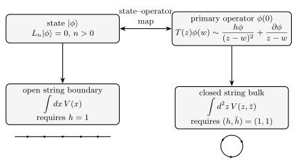
For the level-zero, one and two examples below, the relevant poles have orders one through four. The cubic and quartic coefficients test $L_1$ and $L_2$; the double pole supplies the weight. The counterclockwise contour lies in the doubled holomorphic plane. Its lower half is the reflected continuation of an open-string boundary problem, not an additional physical worldsheet region. Geometry and contour radii are schematic.

The physical quotient is still necessary

The covariant matter Fock space has an indefinite inner product. Define the radical of its restriction to $\mathcal P$ by

$$\mathcal R=\{\,|s\rangle\in\mathcal P: \langle\phi|s\rangle=0\text{ for every }|\phi\rangle\in\mathcal P\,\}.$$

The physical state space is $\mathcal H_{\rm phys}=\mathcal P/\mathcal R$. A zero-self-norm vector is not automatically radical in an arbitrary indefinite space. A useful sufficient construction is a physical spurious state: a sum of negative-mode descendants which also satisfies the physical conditions. For every physical bra,

$$\langle\phi|L_{-n}|\chi\rangle =\langle L_n\phi|\chi\rangle=0\qquad(n>0).$$

It follows that such a sum belongs to $\mathcal R$. Neither an arbitrary descendant nor an arbitrary weight-one operator is thereby declared physically trivial.

There is a distinction from null decoupling in a unitary minimal model. A physical null state need not vanish as a field of the entire timelike matter CFT. It is orthogonal to physical states, and may pair with unphysical ones. The quotient relevant to strings is imposed after the physical conditions. Exercise 3 gives an explicit example.

Boundary doubling and the exact operator map

Let $V_k(t)=:e^{ik\cdot X(t)}:$ on the real boundary of the upper half-plane. In the doubling description, a tangential derivative acts on both equal chiral pieces. Define the local boundary current

$$J^\mu(t)=\partial_tX^\mu(t)=2\partial X_L^\mu(t).$$

The image contraction gives

$$\partial X_L^\mu(z)V_k(t)\sim -\frac{i\alpha'k^\mu}{z-t}V_k(t), \qquad \partial X_L^\mu(z)J^\nu(t)\sim -\frac{\alpha'\eta^{\mu\nu}}{(z-t)^2}.$$

Contracting both fields of $T=-:\partial X_L\cdot\partial X_L:/\alpha'$ with the exponential therefore gives $h_k=\alpha'k^2$. The boundary weight is four times the bulk holomorphic weight because the doubled contraction is squared. This is an application of the image method, not a change of string scale; see Tong’s §5.4.2.

The open oscillator zero mode is $q^\mu=\alpha_0^\mu=\sqrt{2\alpha'}\,k^\mu$. Acting on the momentum vacuum,

$$J^\mu(t)|0;k\rangle =-\frac{2i\alpha'k^\mu}{t}|0;k\rangle -i\sqrt{2\alpha'}\sum_{r\ge1}t^{r-1}\alpha_{-r}^\mu|0;k\rangle.$$

The limit at $t=0$ must subtract the momentum pole. Joint normal ordering does exactly that. Differentiating $m-1$ times then selects the constant creation term with $r=m$, producing

$$\alpha_{-m}^\mu|0;k\rangle \quad\longleftrightarrow\quad \frac{i}{\sqrt{2\alpha'}(m-1)!} :\partial_t^mX^\mu e^{ik\cdot X}:, \qquad m\ge1.$$

For several oscillators multiply these coefficients and place every derivative and the exponential inside a single normal product. This subtracts derivative–derivative and derivative–exponential contractions at the insertion. The coefficient differs from the closed chiral dictionary because $\partial_tX$ differentiates the doubled field.

At oscillator level $N$, the boundary weight is $h=\alpha'k^2+N$. Consequently $h=1$ gives $\alpha'M^2=N-1$. The level-zero exponential is the open tachyon, with $M^2=-1/\alpha'$. Its negative mass squared signals an unstable perturbative vacuum; it does not mean a negative-norm state. A weight eigenoperator at higher level still has to pass the higher-pole test.

The vector vertex and longitudinal gauge states

Consider the boundary field

$$V_\epsilon(t)=:\epsilon\cdot J(t)e^{ik\cdot X(t)}:.$$

It creates $-i\sqrt{2\alpha'}\,\epsilon\cdot\alpha_{-1}|0;k\rangle$. Thus $iV_\epsilon/\sqrt{2\alpha'}$ is the exact representative of the state with oscillator coefficient $\epsilon$; an overall vertex normalization is otherwise conventional.

A potentially offending stress contraction joins one field in $T$ to $J$ and the other to the exponential. There are two assignments, giving

$$-\frac2{\alpha'} \left(-\frac{\alpha'\epsilon_\mu}{(z-t)^2}\right) \left(-\frac{i\alpha'k^\mu}{z-t}\right)V_k =-\frac{2i\alpha'(k\cdot\epsilon)}{(z-t)^3}V_k.$$

The remaining contractions and Taylor terms give the full singular OPE:

$$T(z)V_\epsilon(t)\sim -\frac{2i\alpha'(k\cdot\epsilon)V_k}{(z-t)^3} +\frac{(1+\alpha'k^2)V_\epsilon}{(z-t)^2} +\frac{\partial_tV_\epsilon}{z-t}.$$

The weight-one primary conditions are therefore $k^2=0$ and $k\cdot\epsilon=0$. The cubic coefficient of the exactly normalized state representative is $q\cdot\epsilon$, in agreement with $L_1\epsilon\cdot\alpha_{-1}|0;k\rangle$.

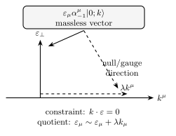
At nonzero null momentum, transversality leaves $k^\perp$, which still contains $k$ itself. The longitudinal state is

$$L_{-1}|0;k\rangle=q\cdot\alpha_{-1}|0;k\rangle, \qquad k^2=0.$$

The seed has weight zero, and $L_1L_{-1}|0;k\rangle=2L_0|0;k\rangle=0$. Higher positive modes also vanish. The descendant is thus physical, and the adjoint argument puts it in the radical. Hence

$$\epsilon_\mu\sim\epsilon_\mu+\lambda k_\mu, \qquad \mathcal H_{N=1}=k^\perp/\operatorname{span}\{k\}.$$

The quotient has 24 positive polarizations at $D=26$. For example, with $k^\mu=(E,0,\ldots,0,E)$ and $E\ne0$, the constraint gives $\epsilon^{25}=\epsilon^0$; a longitudinal shift sets both to zero. It is the quotient, not transversality alone, that removes this remaining null line.

Integrated longitudinal vertices have endpoint terms

At separated points the corresponding local identity is

$$:k\cdot J e^{ik\cdot X}:=-i\partial_t V_k.$$

It explains the relation to a spacetime gauge shift of the vector potential. It does not yet prove that every integrated correlator vanishes. On a regulated ordered interval $a+\epsilon<t<b-\epsilon$,

$$\int_{a+\epsilon}^{b-\epsilon}dt\, \langle V_k^{\rm long}(t)\,\mathcal O\rangle =-i\left[\langle V_k(t)\,\mathcal O\rangle\right]_{a+\epsilon}^{b-\epsilon}.$$

The endpoint values are essential when $a,b$ are other punctures. They vanish in a suitable convergence domain, or may cancel after the full amplitude prescription is applied. Singular contacts, boundaries of moduli space, or an incomplete integration domain cannot be discarded merely by calling the insertion a total derivative.

A concrete local example is $F(t)=t^u(1-t)^v$ on $0<t<1$. Such powers arise from contractions of $V_k$ with vertices at 0 and 1; in that application $u=2\alpha'k\cdot p_0$ and $v=2\alpha'k\cdot p_1$. For $\operatorname{Re}u,\operatorname{Re}v>0$, both endpoint terms vanish as the cuts close. The corresponding beta-function identity and a counterexample outside that region are derived in exercise 4. Analytic continuation of a complete string amplitude is a further step, not evaluation of divergent endpoint expressions.

The example is $F(t)=t(1-t)^2$ with dimensionless $t$ and cuts at $\epsilon=0.1$ and $1-\epsilon=0.9$. Its regulated derivative integral is $0.009-0.081=-0.072$, approaching zero only when the cuts close. For general complex powers, vanishing of each endpoint requires $\operatorname{Re}u,\operatorname{Re}v>0$. The shading marks the regulated coordinate domain; the area under F is not the integral of F′. The curve illustrates the local integral, not a complete string amplitude or a claim that contact terms always vanish.

The first massive vertex and its higher poles

At open level two, take the oscillator state

$$|\Psi;k\rangle= \left(S_{\mu\nu}\alpha_{-1}^\mu\alpha_{-1}^\nu +v_\mu\alpha_{-2}^\mu\right)|0;k\rangle, \qquad S_{\mu\nu}=S_{\nu\mu}.$$

There is no factor $1/2$ before $S$. The boundary dictionary gives its exact field:

$$\mathcal V_{S,v} =:\left[-\frac{S_{\mu\nu}}{2\alpha'}J^\mu J^\nu +\frac{i v_\mu}{\sqrt{2\alpha'}}\partial_tJ^\mu\right]e^{ik\cdot X}:.$$

Its weight is $h=2+\alpha'k^2$. Before imposing any constraints, the stress OPE is

$$T(z)\mathcal V_{S,v}(t)\sim \frac{\mathcal A_2(t)}{(z-t)^4} +\frac{\mathcal A_1(t)}{(z-t)^3} +\frac{h\mathcal V_{S,v}(t)}{(z-t)^2} +\frac{\partial_t\mathcal V_{S,v}(t)}{z-t},$$

where

$$\begin{aligned} \mathcal A_2&=(S^\mu{}_{\mu}+2q\cdot v)V_k,\\ \mathcal A_1&=\frac{2i}{\sqrt{2\alpha'}} (S_{\mu\nu}q^\nu+v_\mu):J^\mu e^{ik\cdot X}:. \end{aligned}$$

These coefficients can be obtained without assuming the oscillator result. For the quartic pole, contracting the two stress fields with the two $J$ fields gives $S^\mu{}_{\mu}$. The mixed contraction with $\partial_tJ$ and the exponential gives the other term: differentiating the second basic contraction above yields $-2\alpha'/(z-t)^3$, so

$$\left(-\frac2{\alpha'}\right) \left(-\frac{2\alpha'v_\mu}{(z-t)^3}\right) \left(-\frac{i\alpha'k^\mu}{z-t}\right) \frac{i}{\sqrt{2\alpha'}} =\frac{2q\cdot v}{(z-t)^4}.$$

For the cubic pole, there are four mixed contractions involving one of the two $J$ fields and the exponential. They leave $2i S_{\mu\nu}k^\nu J^\mu V_k$. A single contraction with $\partial_tJ$ leaves $2i v_\mu J^\mu V_k/\sqrt{2\alpha'}$. Together they give $\mathcal A_1$. The lower poles follow from the remaining contractions and Taylor expansion. No pole above order four is possible in this product.

Requiring a weight-one primary gives

$$q^2=-2, \qquad S_{\mu\nu}q^\nu+v_\mu=0, \qquad S^\mu{}_{\mu}+2q\cdot v=0.$$

The mass shell is $M^2=1/\alpha'$. As an independent check, the oscillator commutators yield

$$\begin{aligned} L_1|\Psi;k\rangle&=2(S_{\mu\nu}q^\nu+v_\mu) \alpha_{-1}^\mu|0;k\rangle,\\ L_2|\Psi;k\rangle&=(S^\mu{}_{\mu}+2q\cdot v)|0;k\rangle. \end{aligned}$$

The exact boundary dictionary maps these two states into $\mathcal A_1$ and $\mathcal A_2$. The operator and oscillator tests have therefore imposed the same conditions, including all factors.

Vector null descendants

Let $|\chi_e\rangle=e\cdot\alpha_{-1}|0;k\rangle$ with $q^2=-2$ and $q\cdot e=0$. It is a primary of weight zero. Its derivative $L_{-1}|\chi_e\rangle$ is a physical weight-one descendant. In the $(S,v)$ description it shifts

$$\delta S_{\mu\nu}=q_{(\mu}e_{\nu)}, \qquad \delta v_\mu=e_\mu, \qquad q\cdot e=0,$$

where symmetrization has weight $1/2$. Substitution into both constraints makes them vanish. Its field is the derivative of the weight-zero seed field, and is orthogonal to all physical states by the same adjoint argument as the vector’s longitudinal state.

The scalar null at the critical central charge

There is also a scalar candidate

$$|s\rangle=\left(L_{-2}+\frac32L_{-1}^2\right)|0;k\rangle, \qquad L_0|0;k\rangle=-|0;k\rangle.$$

It is a weight-one descendant of a weight-minus-one seed. The Virasoro algebra explains the coefficient $3/2$:

$$L_1L_{-2}|0;k\rangle=3L_{-1}|0;k\rangle, \qquad L_1L_{-1}^2|0;k\rangle=-2L_{-1}|0;k\rangle.$$

Those contributions cancel. The independent $L_2$ test gives

$$L_2|s\rangle=\frac{D-26}{2}|0;k\rangle.$$

At $D=26$ the candidate is physical and lies in the radical. Higher positive modes vanish by level counting. Exercise 5 derives its norm and explains why a negative value away from the critical dimension would not, by itself, be a physical ghost.

The local field is also explicit. The regular term of $T(z)V_k(t)$ defines $L_{-2}V_k$. Taylor-expanding the uncontracted stress current gives

$$L_{-2}V_k=:\left[-\frac{J^2}{4\alpha'}+i k\cdot\partial_tJ\right]e^{ik\cdot X}:, \qquad L_{-1}^2V_k=\partial_t^2V_k.$$

Since $\partial_t^2V_k=:[i k\cdot\partial_tJ-(k\cdot J)^2]e^{ik\cdot X}:$, the scalar representative is

$$\mathcal V_s=:\left[-\frac{J^2}{4\alpha'} +\frac{5i}{2}k\cdot\partial_tJ -\frac32(k\cdot J)^2\right]e^{ik\cdot X}:.$$

This is generally a nonzero matter operator. At $D=26$, its higher stress poles vanish, and its state is removed by the physical null quotient. The descendant $L_{-2}V_k$ alone fails the $L_1$ test; the $(3/2)\partial_t^2V_k$ contribution is essential.

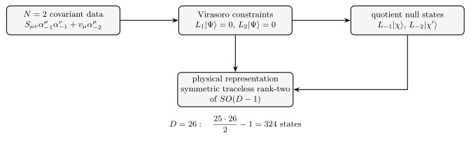
The seed has $h_0=-1$, and the matter central charge is $c=D$. The coefficients $+3$ and $-3$ cancel in $L_1(L_{-2}+\tfrac32L_{-1}^2)|h_0\rangle$. The remaining $L_2$ coefficient is $(D-26)/2$. At $D=26$ the descendant is a physical radical vector; the diagram describes mode actions and is not a count of the whole massive spectrum.

The massive physical representative

The scalar null changes the oscillator coefficients by

$$\delta S_{\mu\nu}=\lambda\left(\frac12\eta_{\mu\nu} +\frac32q_\mu q_\nu\right), \qquad \delta v_\mu=\frac52\lambda q_\mu.$$

Together with the vector nulls it can set $v'=0$. For example, choose $\lambda=(v\cdot q)/5$ and $e_\mu=-v_\mu-(v\cdot q)q_\mu/2$. The remaining physical conditions are then

$$S'_{\mu\nu}q^\nu=0, \qquad S'^\mu{}_{\mu}=0.$$

In the massive rest frame $S'$ has only spatial components. Its norm is $2\sum_{i,j=1}^{25}|S'_{ij}|^2$, and its representation is the symmetric traceless tensor of $SO(25)$, of dimension 324. The complete uniqueness and counting argument is on page 07; exercise 2 below recovers the same positive pairing from the vertex two-point function. The scalar reduction used here is specifically the critical one.

Closed massless vertices and the transverse trace

For a closed string, the exact representative of $E_{\mu\nu}\alpha_{-1}^\mu\widetilde\alpha_{-1}^\nu|0;k\rangle$ is

$$\mathcal U_E=-\frac2{\alpha'} E_{\mu\nu}:\partial X^\mu\bar\partial X^\nu e^{ik\cdot X}:.$$

The unscaled tensor operator’s holomorphic cubic stress coefficient is

$$-\frac{i\alpha'}2k^\mu E_{\mu\nu} :\bar\partial X^\nu e^{ik\cdot X}:,$$

with an independent barred coefficient contracting the other index. Thus the $(1,1)$ primary conditions are $k^2=0$, $k^\mu E_{\mu\nu}=0$ and $E_{\mu\nu}k^\nu=0$. The full Wick derivation is on page 12. Matter primarity still admits the physical gauge shifts

$$E_{\mu\nu}\sim E_{\mu\nu}+k_\mu\lambda_\nu +\widetilde\lambda_\mu k_\nu, \qquad k\cdot\lambda=k\cdot\widetilde\lambda=0.$$

At nonzero null momentum choose another null vector $\ell$ with $k\cdot\ell=-1$. The projector

$$P_{\mu\nu}=\eta_{\mu\nu}+k_\mu\ell_\nu+\ell_\mu k_\nu$$

has rank $d=D-2$, annihilates $k$ and $\ell$, and selects a Euclidean transverse space. In a transverse basis the physical tensor is a matrix $E_{ij}$, with

$$E_{ij}=\left(E_{(ij)}-\frac{t}{d}\delta_{ij}\right) +E_{[ij]}+\frac{t}{d}\delta_{ij}, \qquad t=\delta^{ij}E_{ij}.$$

The three pieces are the graviton, two-form and scalar dilaton polarizations. For $D=26$ their dimensions are $299+276+1=576$. The normalized scalar representative is $P_{\mu\nu}/\sqrt{24}$. A bare $\eta_{\mu\nu}$ fails the transverse condition, so subtracting its Lorentz trace with denominator $D$ would not give three separately physical pieces. The identification of this scalar with a particular spacetime dilaton variable also involves the low-energy field definitions.

In the unwound noncompact theory, the two zero-mode equations give $N=\widetilde N$. Compact momentum and winding modify their difference, as explained on page 06; they are not included in this massless example. Integrated pure-gauge bulk vertices are total derivatives away from contacts, subject to the same amplitude qualifications as the boundary case. Their spacetime interpretation is developed further on page 22.

What the no-ghost theorem establishes

The low-level calculations above show how positive physical pairings emerge, but do not prove positivity at every oscillator level. The no-ghost theorem of Brower and Goddard and Thorn supplies the all-level result. For the critical free bosonic string with one timelike coordinate, $D=26$, intercept one and nonzero momentum, the constrained space is positive semidefinite, and

$$\mathcal P/\mathcal R\cong\mathcal F_{24}^{\rm transverse}$$

at each corresponding mass level. Closed strings use both chiral sectors with level matching. The ordinary light-cone description chooses a frame with $k^+\ne0$; for nonzero momentum an appropriate null direction can be chosen. This is an isomorphism of physical state spaces and inner products, not an identification of each covariant oscillator with a transverse oscillator.

The theorem requires a completeness argument at arbitrary level, which is not derived here. Constructing positive physical states alone would not exclude additional negative-norm states outside that construction. The spectrum-generating approach establishes the necessary completeness; the explicit low-level null and OPE calculations illustrate the result rather than replacing its proof.

At exactly $k=0$, the level-one timelike state $\alpha_{-1}^0|0;0\rangle$ satisfies the displayed old covariant conditions and has norm $-1$. The longitudinal descendant $k\cdot\alpha_{-1}|0;0\rangle$ is zero. Such exceptional momentum sectors are outside the ordinary propagating-polarization assertion above and require separate treatment.

Finally, free-state positivity alone does not uniquely determine the critical interacting theory. In the usual integer-dimensional old covariant model, the wider free no-ghost range includes $2\le D\le25$, $a\le1$, in addition to $D=26,a=1$; it does not include every pair with $D\le26,a\le1$. The additional longitudinal state content and distinction from the critical transverse theory are discussed by Daszkiewicz, Hasiewicz and Jaskólski, §2. Page 07 gives a direct counterexample at $D=26,a=1/2$. Consistency of the full matter-plus-ghost theory, vacuum stability and the interacting amplitudes are further requirements.

Exercises

1. A higher boundary oscillator is not automatically primary

Derive the exact operators for $\alpha_{-3}^\mu|0;k\rangle$ and $\alpha_{-2}^\mu\alpha_{-1}^\nu|0;k\rangle$. At $k=0$, calculate the singular OPE of $T(z)$ with $\partial_t^2J^\mu(t)$. Check its two higher poles against the oscillator actions.

Solution

Subtract the momentum pole in $J(t)|k\rangle$ before differentiating. Two derivatives select $2!\,\alpha_{-3}$, whereas one derivative selects $\alpha_{-2}$. Joint normal ordering gives

$$\begin{aligned} \alpha_{-3}^\mu|0;k\rangle &\longleftrightarrow\frac{i}{2\sqrt{2\alpha'}}:\partial_t^2J^\mu e^{ikX}:,\\ \alpha_{-2}^\mu\alpha_{-1}^\nu|0;k\rangle &\longleftrightarrow-\frac1{2\alpha'}:\partial_tJ^\mu J^\nu e^{ikX}:. \end{aligned}$$

Separate normal ordering of the factors would fail to remove all coincident contractions in the second expression.

At zero momentum, $J$ is primary of weight one. Differentiate its stress OPE twice with respect to the insertion coordinate:

$$T(z)\partial_t^2J(t)\sim \frac{6J(t)}{(z-t)^4} +\frac{6\partial_tJ(t)}{(z-t)^3} +\frac{3\partial_t^2J(t)}{(z-t)^2} +\frac{\partial_t^3J(t)}{z-t}.$$

The weight is three, but the higher poles make it nonprimary. Multiplying by the exact coefficient $i/(2\sqrt{2\alpha'})$, the quartic pole creates $3\alpha_{-1}|0;0\rangle$ and the cubic pole creates $3\alpha_{-2}|0;0\rangle$. These agree with $L_2\alpha_{-3}|0;0\rangle=3\alpha_{-1}|0;0\rangle$ and $L_1\alpha_{-3}|0;0\rangle=3\alpha_{-2}|0;0\rangle$. The factorial is essential for this check.

2. Recover the massive positive pairing from two vertices

Take the critical massive representative with $v=0$, $k^2=-1/\alpha'$, $S_{\mu\nu}k^\nu=0$ and $S^\mu{}_{\mu}=0$. Evaluate the boundary two-point function of its exact vertex and the opposite-momentum vertex with polarization $S^*$. Strip the momentum-conserving delta function and use unit vacuum normalization. Recover the oscillator pairing.

Solution

Each vertex has coefficient $-1/(2\alpha')$. Derivative contractions with the other exponential vanish by $S_{\mu\nu}k^\nu=0$. Self-contractions are absent by joint normal ordering. The two complete pairings of the derivative fields give

$$\langle\mathcal V_{S^*}(-k;t)\mathcal V_S(k;0)\rangle_{\rm stripped} =\frac1{4\alpha'^2}\,2\frac{(2\alpha')^2}{t^4} S^*_{\mu\nu}S^{\mu\nu}\,|t|^{-2\alpha'k^2}.$$

For $t>0$, the last factor is $t^2$. Thus

$$\langle\mathcal V_{S^*}(-k;t)\mathcal V_S(k;0)\rangle_{\rm stripped} =\frac{2S^*_{\mu\nu}S^{\mu\nu}}{t^2}.$$

This is a weight-one primary pairing. With the radial-conjugation prescription of page 13, its coefficient is the state norm. In the massive rest frame transversality removes all time indices, leaving $2\sum_{i,j=1}^{25}|S_{ij}|^2$. Its positivity follows from the physical representative, not from positivity of the unrestricted covariant matter CFT.

3. A physical null field need not vanish in the matter CFT

Let $k$ be nonzero and null, and choose a null $\ell$ with $k\cdot\ell=-1$. Compare the states $|g\rangle=k\cdot\alpha_{-1}|0;k\rangle$ and $|u\rangle=\ell\cdot\alpha_{-1}|0;k\rangle$. Compute their self-pairings and mutual pairing, and identify which state is physical. Explain why the gauge field cannot be set to zero as an identity of the whole matter operator algebra. Contrast the exactly zero-momentum level-one sector.

Solution

The oscillator Gram form is the Lorentz metric, so

$$\langle g|g\rangle=k^2=0, \qquad \langle u|u\rangle=\ell^2=0, \qquad \langle u|g\rangle=\ell\cdot k=-1.$$

Both states have $L_0=1$, but only $g$ passes transversality:

$$L_1|g\rangle=0, \qquad L_1|u\rangle=-\sqrt{2\alpha'}\,|0;k\rangle.$$

Thus $g$ is orthogonal to every physical state but pairs nontrivially with an unphysical state. The two-dimensional ambient Gram matrix is $\left(\begin{smallmatrix}0&-1\\-1&0\end{smallmatrix}\right)$, which is nondegenerate and indefinite. The local field corresponding to $g$ is a nonzero derivative of $V_k$; it is removed in the physical quotient, not declared zero in the full free-boson CFT.

At $k=0$, every level-one polarization obeys the positive-mode constraints, while $L_{-1}|0;0\rangle=0$. In particular, the state $\alpha_{-1}^0|0;0\rangle$ has norm $-1$ and is not removed by that longitudinal construction. This is why the nonzero-momentum condition is part of the ordinary no-ghost/polarization statement.

4. A regulated gauge integral and its convergence domain

For $F(t)=t^u(1-t)^v$, compute $\int_0^1F'(t)dt$ where both differentiated terms are integrable. Derive the beta-function identity. For $u=1,v=2$, evaluate the integral with cuts at $0.1$ and $0.9$. Then repeat the endpoint analysis for $u=0,v=1$ and for $u=-1,v=1$.

Solution

For $\operatorname{Re}u,\operatorname{Re}v>0$,

$$\int_0^1F'(t)dt =u B(u,v+1)-v B(u+1,v).$$

Using $B(a,b)=\Gamma(a)\Gamma(b)/\Gamma(a+b)$, both terms are $\Gamma(u+1)\Gamma(v+1)/\Gamma(u+v+1)$, so their difference vanishes. This agrees with both endpoints of $F$ tending to zero.

At $u=1,v=2$, $F(t)=t-2t^2+t^3$ and $F'(t)=1-4t+3t^2$. The regulated answer is

$$\int_{0.1}^{0.9}F'(t)dt =0.9(0.1)^2-0.1(0.9)^2=-0.072.$$

It is nonzero before the cuts close. At $u=0,v=1$, $F=1-t$ has a nonzero lower endpoint, so the full derivative integral equals $-1$. At $u=-1,v=1$, $F=1/t-1$, and

$$F(1-\epsilon)-F(\epsilon) =\frac1{1-\epsilon}-\frac1\epsilon$$

diverges as $\epsilon\to0$. A total derivative therefore does not justify dropping endpoint terms for arbitrary exponents. The beta identity has a meromorphic analytic continuation, but that continued identity is not the value of these unregulated divergent integrals. In a string amplitude one must specify the complete analytic-continuation and contact prescription.

5. Derive the scalar null and test its descendants

For a highest-weight seed $|h\rangle$, derive the $2\times2$ Gram matrix of $L_{-2}|h\rangle$ and $L_{-1}^2|h\rangle$. Set $h=-1$, $c=D$, and use it to find the norm of $|s\rangle=(L_{-2}+\tfrac32L_{-1}^2)|h\rangle$. At $D=26$, is $L_{-1}|s\rangle$ another physical state at the same momentum?

Solution

The adjoint and Virasoro algebra give

$$M_2=\begin{pmatrix} 4h+c/2&6h\\ 6h&4h(2h+1) \end{pmatrix}.$$

For example, the off-diagonal entry follows from $L_2L_{-1}^2|h\rangle=6h|h\rangle$; the lower diagonal follows by applying $L_1$ twice. At $h=-1$,

$$M_2=\begin{pmatrix}D/2-4&-6\\-6&4\end{pmatrix}, \qquad \langle s|s\rangle =(1,\tfrac32)M_2\begin{pmatrix}1\\3/2\end{pmatrix} =\frac{D-26}{2}.$$

The $L_1$ coefficient is $3+(3/2)(4h+2)=0$, while the $L_2$ coefficient is $4h+D/2+9h=(D-26)/2$. At $D=26$ the state is physical and radical. At $D<26$ its norm is negative but its $L_2$ constraint fails, so it is not a counterexample to a no-ghost theorem.

At the critical value, $s$ has weight one. Its derivative has weight two and

$$L_1L_{-1}|s\rangle=2L_0|s\rangle=2|s\rangle.$$

The derivative has zero self-norm, since $\langle s|s\rangle=0$, but it is not a physical state at the same momentum: both its weight and its positive-mode test fail in the unquotiented matter space. Descendants of a singular vector can inherit zero pairings without satisfying the physical string conditions at their new level. This separates a Virasoro submodule statement from the fixed-mass physical quotient.

6. Normalize the closed scalar vertex and change its reference vector

At nonzero null $k$, use $P_{\mu\nu}=\eta_{\mu\nu}+k_\mu\ell_\nu+\ell_\mu k_\nu$ with $\ell^2=0$, $k\cdot\ell=-1$. Show that $E^{(\Phi)}=P/\sqrt{D-2}$ has unit norm and no cubic stress pole. Derive the two-point coefficient for the exact closed tensor vertex. Finally show that replacing $\ell$ by another allowed reference changes only the gauge representative.

Solution

Contraction with $k$ gives $k^\mu P_{\mu\nu}=k_\nu-k_\nu=0$, and similarly $P\ell=0$. Direct multiplication yields $P^2=P$ and $\operatorname{tr}P=D-2$. Hence

$$E^{(\Phi)}_{\mu\nu}E^{(\Phi)\mu\nu} =\frac{\operatorname{tr}P^2}{D-2}=1.$$

Transversality removes both cubic stress poles. A bare Lorentz-metric polarization would instead give $k^\mu\eta_{\mu\nu}=k_\nu\ne0$.

For two transverse tensors at opposite null momentum, derivative–exponential cross-contractions vanish. One holomorphic and one antiholomorphic derivative contraction remain. Including the exact vertex coefficient $-2/\alpha'$ gives

$$\langle\mathcal U_{E^*}(-k;z,\bar z)\mathcal U_E(k;0)\rangle_{\rm stripped} =\frac4{\alpha'^2}\frac{\alpha'^2}{4|z|^4} E^*_{\mu\nu}E^{\mu\nu} =\frac{E^*_{\mu\nu}E^{\mu\nu}}{|z|^4}.$$

The scalar therefore has unit two-point coefficient, matching its oscillator norm. This calculation is at separated points; mixed contact subtractions belong to the joint composite definition.

For another allowed $\ell'$, let $r=\ell'-\ell$. Then $k\cdot r=0$ and

$$P'_{\mu\nu}-P_{\mu\nu}=k_\mu r_\nu+r_\mu k_\nu.$$

This is exactly a constraint-preserving gauge shift. Its pairing with any transverse physical tensor vanishes. Different reference vectors select different covariant representatives of the same physical scalar, while the three transverse little-group components remain graviton, two-form and dilaton.

References

• Richard C. Brower, “Spectrum-Generating Algebra and No-Ghost Theorem for the Dual Model,” Physical Review D 6 (1972), 1655–1662. doi:10.1103/PhysRevD.6.1655.
• Marcin Daszkiewicz, Zbigniew Hasiewicz and Zbigniew Jaskólski, “Free Strings in Non-Critical Dimensions,” contribution to the NATO Advanced Research Workshop New Developments in Quantum Field Theory, Zakopane, 14–20 June 1997, ITPUWr 916/97. arXiv:hep-th/9712207, §2.
• Peter Goddard and Charles B. Thorn, “Compatibility of the Dual Pomeron with Unitarity and the Absence of Ghosts in the Dual Resonance Model,” Physics Letters B 40 (1972), 235–238. doi:10.1016/0370-2693(72)90420-0.
• David Tong, Lectures on String Theory, University of Cambridge lecture notes (2009; revised 2012). arXiv:0908.0333, §§5.4–5.4.3.